Week 4 - CHT Analysis on Exhaust port

AIM: To perform conjugate heat transfer analysis on Exhaust ports.

INTRODUCTION AND THEORY:

What is Conjugate heat transfer (CHT)

• CHT stands for Conjugate heat transfer.
• Conjugate heat transfer corresponds to the heat transfer in solids and fluids simulatenously. In solids conduction is more dominant whereas in fluids convection is more dominant.
• HEAT TRANSFER IN SOLIDS:
  • In solids, generally the heat transfer occurs by conduction. The heat transfer in solid is expressed by the fouriers law for conductive heat flux.
  • Heat flux is directly proportional to temperature gradient.
  • 
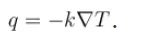
  • In case of solids, convection is not possible because in order for convection to take place the molecules need to move like in liquids and gases. Since, molecules are densly packed in solids, it is not possible for convective heat transfer.
• HEAT TRANSFER IN FLUIDS:
• In fluids, due to its motion there are three contributing factors for heat transfer.
  • Fluid motion contributes to energy transfer which appears in the heat transfer equation as the convective contribution. Depending upon the temperature of the fluid and the fluid regime, the flow can be convective or conductive.
  • The viscous effects of the fluid flow produce fluid heating. This term is often neglected, nevertheless, its contribution is noticeable for fast flow in viscous fluids.
  • As soon as a fluid density is temperature-dependent, a pressure work term contributes to the heat equation. This accounts for the well-known effect that, for example, compressing air produces heat.
• APPLICATIONS OF CHT:
  
  • Effective heat transfer:
    • CHT plays a big role in efficient heat transfer in case of heat exchangers, coolers etc.
    • The fluid usually plays the role of energy carrier on large distances. Forced convection is the most common way to achieve high heat transfer rate. In some applications, the performances are further improved by combining convection with phase change (for example liquid water to vapor phase change).
    • Even so, solids are also needed, in particular to separate fluids in a heat exchanger so that fluids exchange energy without being mixed.
    • Used in heat sinks: Heat sinks are usually made of metal with high thermal conductivity (e.g. copper or aluminum). They dissipate heat by increasing the exchange area between the solid part and the surrounding fluid.
  • Energy saving:
    • Heat transfer in fluids and solids can also be combined to minimize heat losses in various devices.

GEOMETRY SETUP AND SOLVING:

GEOMETRY CLEANUP:

• We will open ANSYS workbench and import the geometry onto the spaceclaim.

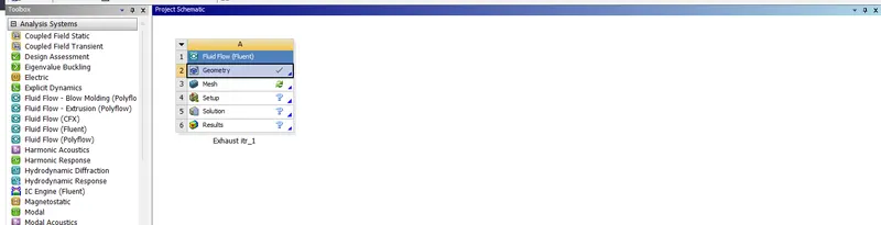
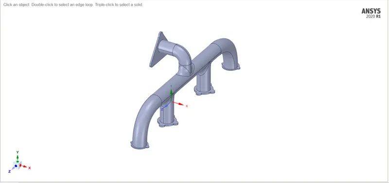
• Once the geometry has been uploaded to Spaceclaim, we need to seperate the internal volume. To do that we will use the volume extract feature to extract the internal volume.
• But before that, we will go to the REPAIR tab and select Extra edges to check for all the extra edges present in the model.

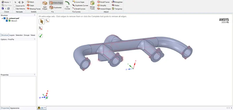
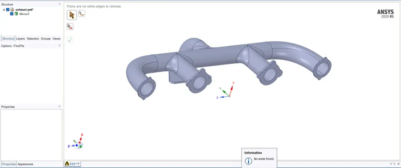
• We will now use the volume extract feature to extract the internal volume.

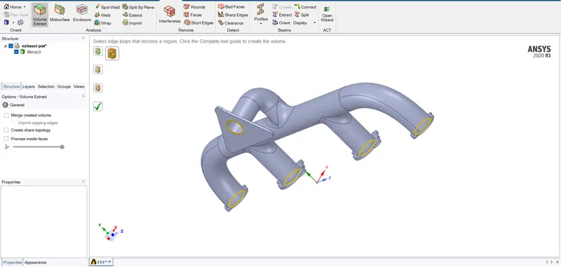
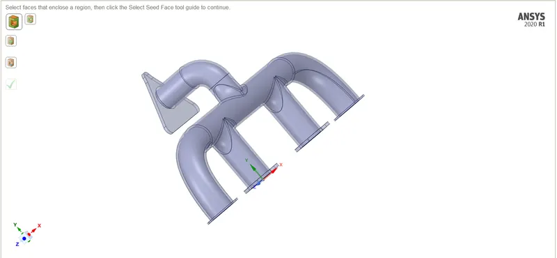
• We can see that an internal volume has been created by ANSYS. We will name the internal volume as fluid-volume and the external enclosure as solid-volume.

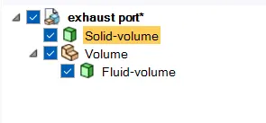
• We will select both the volumes and create a component and then delete the un-necessary components.

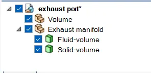
• We need to set the share topology feature to share before moving to the mesh.

• We will go to the workbench tab and perform share.

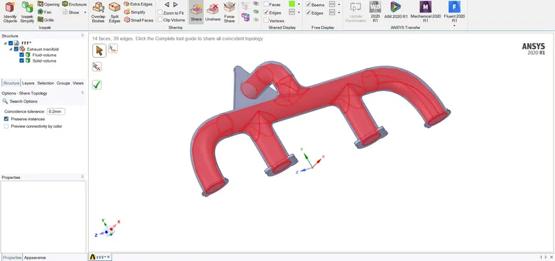
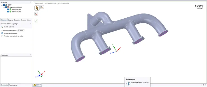
• We can now move to meshing to give named selection and provide the mesh.

MESHING:

Baseline mesh:

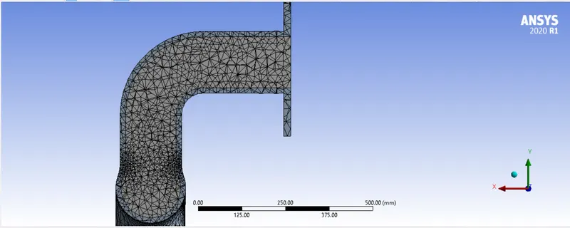
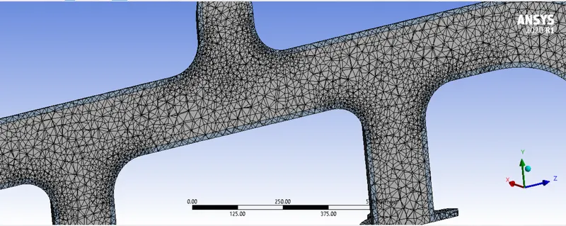
• We will first use a baseline mesh with the default mesh to validate whether the solution is correct or not. We will be trying th analyse the conjugate heat transfer that occurs from the fluid volume to solid volume.
• The solid volume is constructed of Aluminium and the fluid volume has air at high temperature passing through it.
• Through this analysis, we will also conduct a test to which turbulence model to go for.

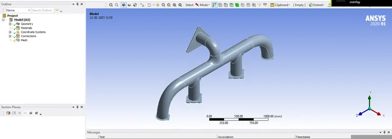
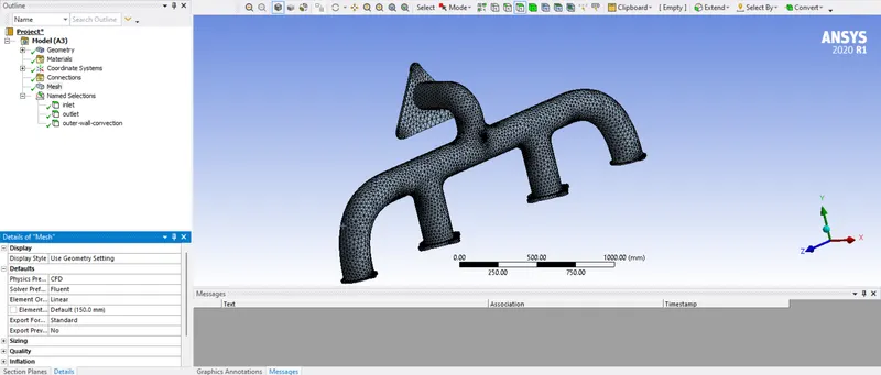
• In the above given image, we can view the model imported into the meshing module.
• We will provide named selection and create a default mesh for analysis.

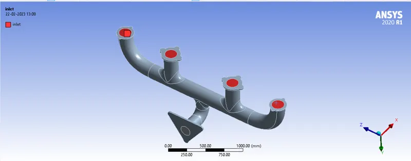
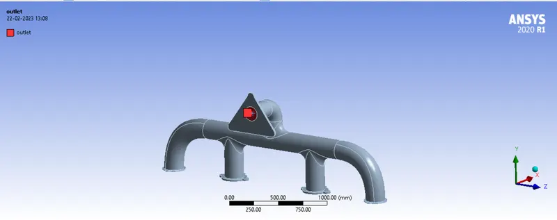
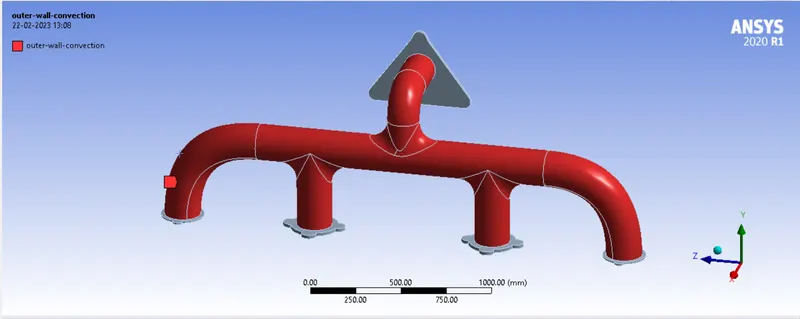
NOTE: The flanges do need to be assigned any named selection as the flanges will be not be participating in heat transfer.

• After the named selections have been created, we can mesh the geometry.

FLUENT:

• First we will check the mesh in Fluent.
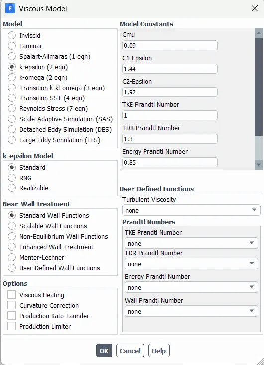
• After that we will move to the physics window and turn the energy mode on. We will be using the RANS model and try to determine which model to use k-epsilon or k-omega.
• First we will select the k-epsilon model.

K-EPSILON MODEL:

• For the solid volume we will be using aluminum and for the fluid volume we will be using air. We need to make sure the materials are present.

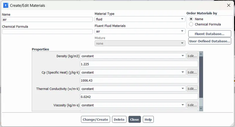
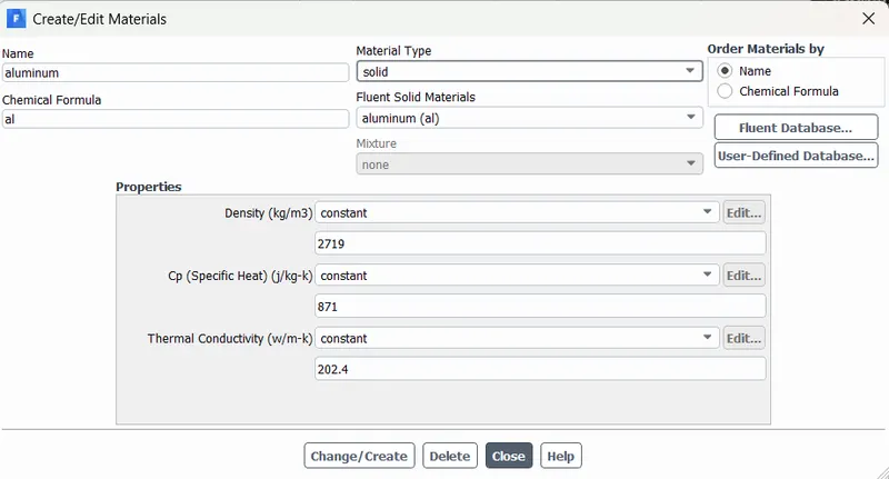
• We will also check whether the correct cell zone conditions are applied.

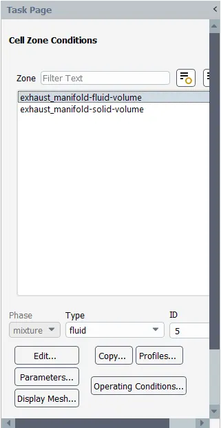
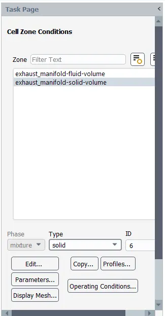
• For the boundary conditions we will set the following

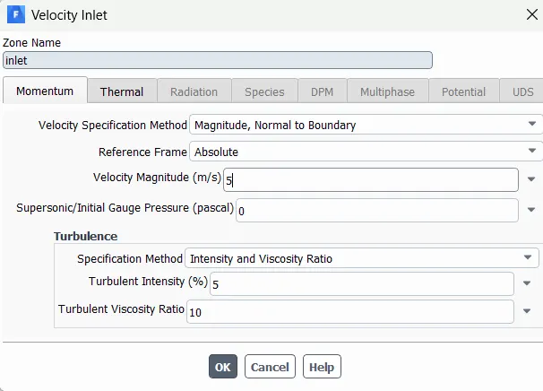
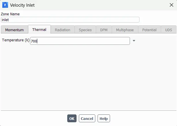
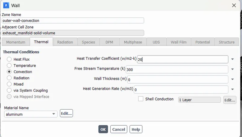
• We will now move to the solution window and select SIMPLE as the solution method.

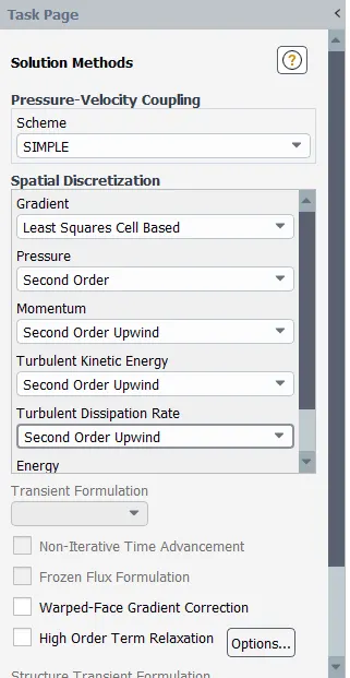
• After the following conditions are set, we will use initialis the analysis and create an temperature plot to understand the results.
• We will run the analysis for 100 iterations.

RESULTS FROM K-EPSILON MODEL:

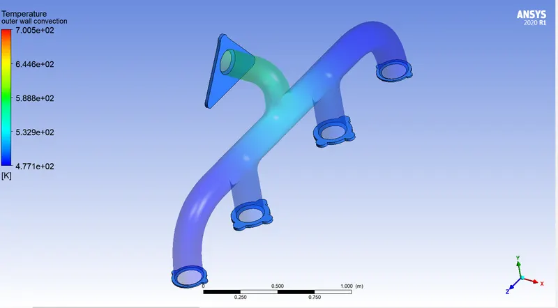
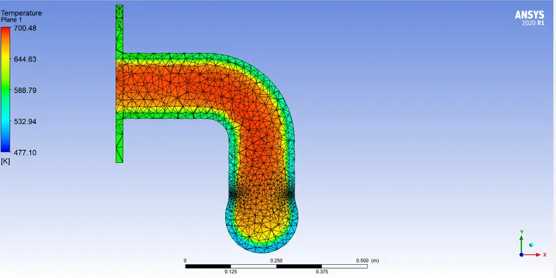
• Temperature plot:

• Velocity plot:

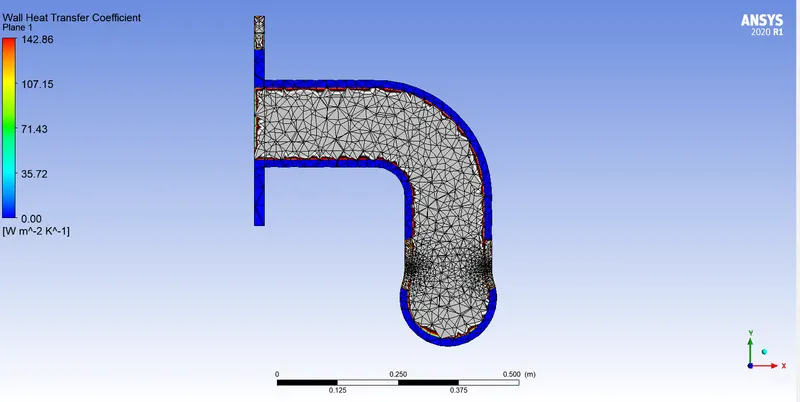
• Heat transfer coeffiecient:

K-OMEGA SST MODEL:

• We will open the setup and select the K-omega model and all the data to be entered is same as the K-epsilon model. We will initialize our model and run calculation.

RESULTS FOR K-OMEGA SST MODEL:

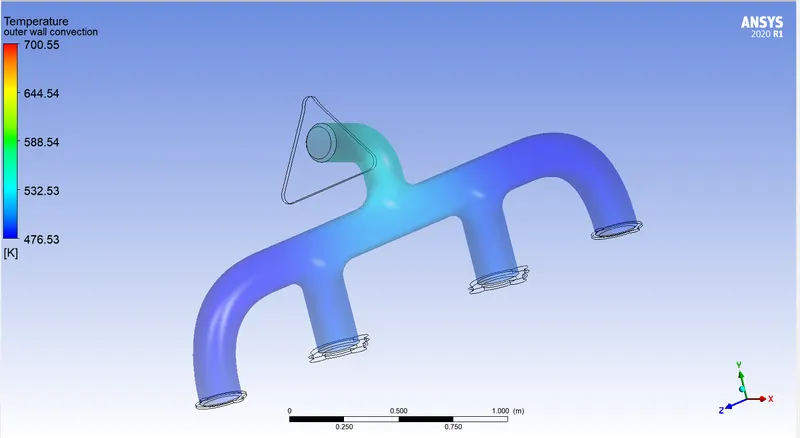
• Temperature contour:

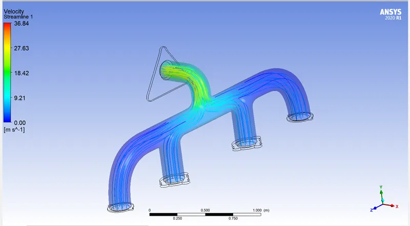
• Velocity contour:

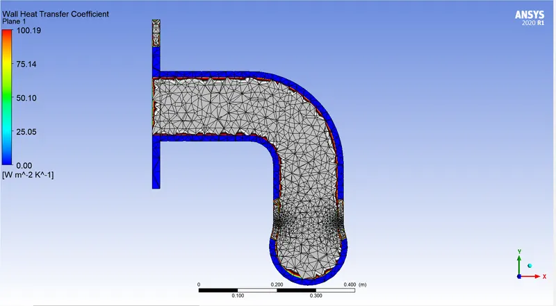
• Heat transfer coefficient:

Analysis from baseline mesh:

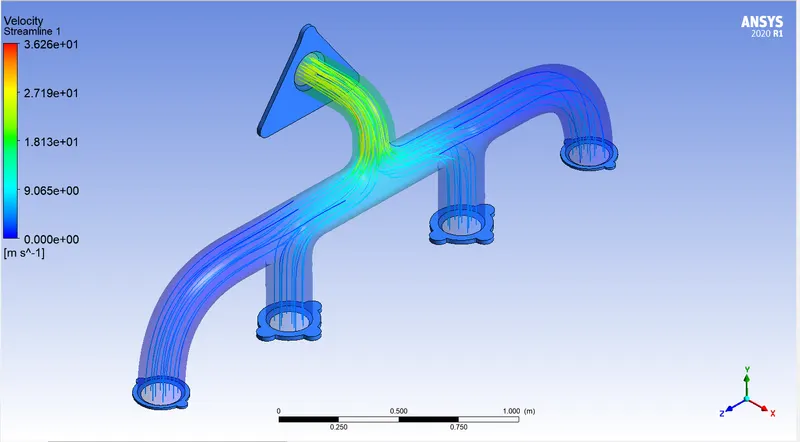
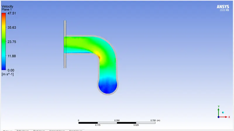
• The reason for increased temperature at the outlet pipe is due to the fact that volume flowing needs to be conserved. Therefore, the volume of fluid flowing at the inlet needs to be equal to the volume of fluid that exits from the outlet. With area being constant, the variable that can be changed is velocity. Thus, there is an increase in velocity at the outlet along with increase in temperature.
• In both the model, if we observe the heat transfer coeffiefient contour. The HTC showed by K-Omega SST is more precise compared to K-epsilon because the K-Omega model is much suited for handling near wall treatment and predicts accurate near wall data.

Conclusion:

• We will be using K-Omega SST as the model for our experiment.
• The K-omega model is a low reynolds number model which is much suited to calculate the flow through the viscous sub-layer. In our case, heat transfer is a problem where the heat transfer coefficient needs to be calculated at the viscous sub layer. Thus, for K-Omega model the y+ value generally needs be less that 5 i.e., (Y+) < 5.
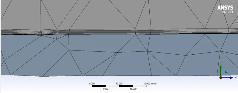
• In order to accurately measure the results near the wall, we need to provide inflation layer to the geometry according to the y+ range suitable for the K-Omega turbulance model.

FINALISED MESH:

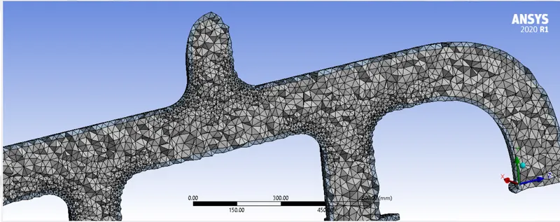
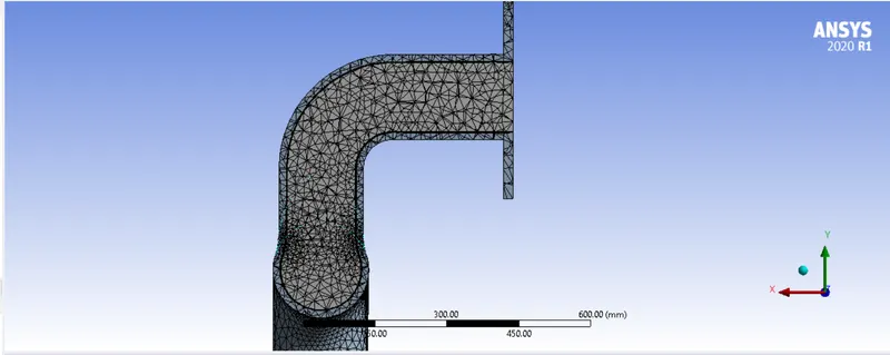
• We will re-mesh the geometry by providing an inflation layer at the internal fluid volume.
• Before that we need to provide a named selection for the internal volume.

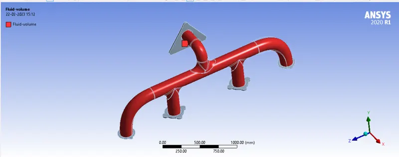
• We will provide an inflation layer by using the first layer thickness which we will calculate by using the Y+ calculator.

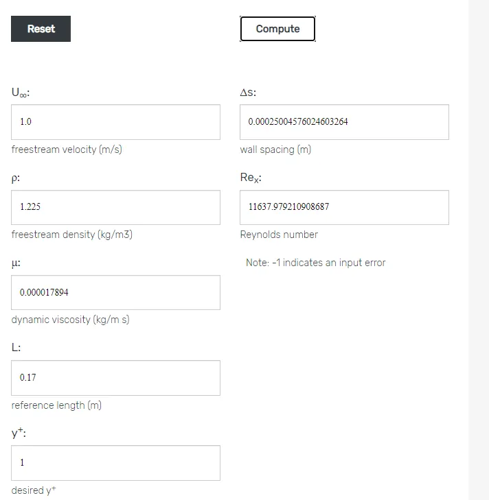
• With the following value for first layer thickness. We will select the fluid volume and give the inflation layer.

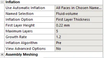
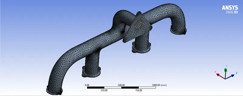
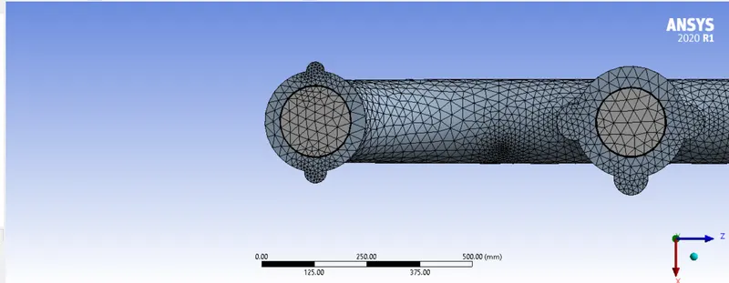
• We will generate the mesh and keep the mesh length as 100mm.

ANALYSIS:

• For the analysis section we will set the model to be K-Omega SST, apart from that all the other aspects of the input data are same.
• While solving for results, this time we will also plot other contours to get a more detailed view of out experiments.

RESULTS:

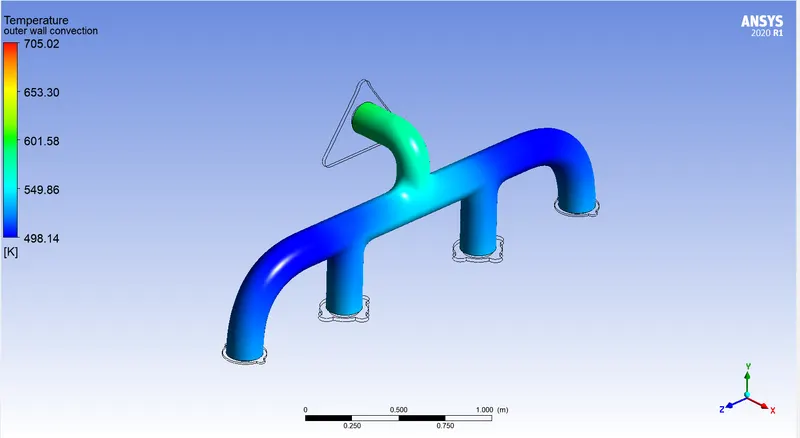
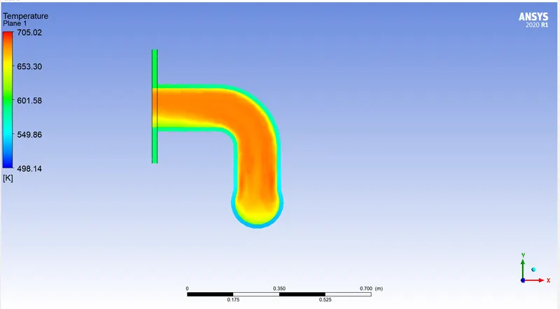
• Temperature contour:

• Velocity contour:

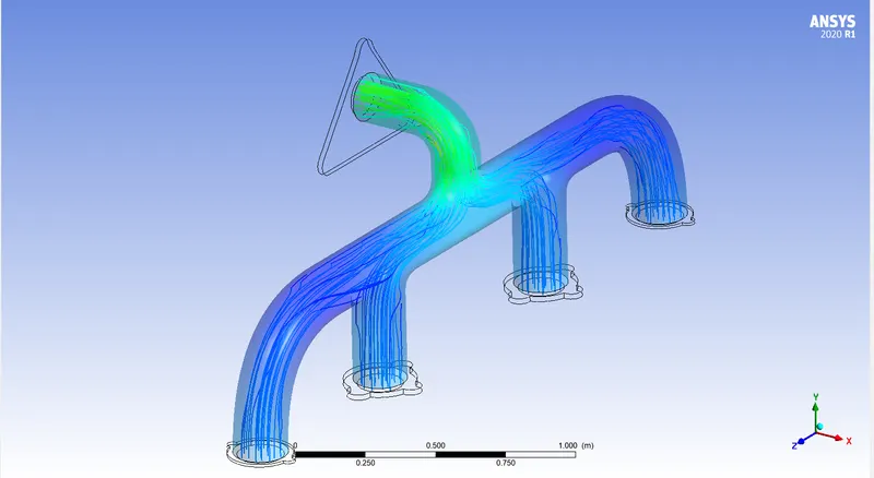
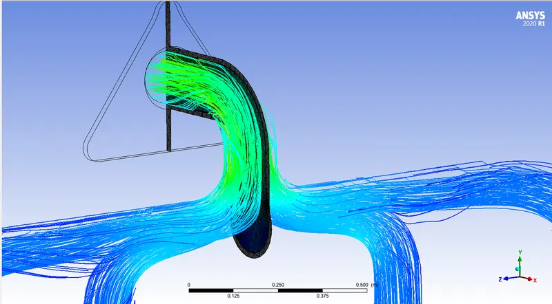
• Velocity steamline:

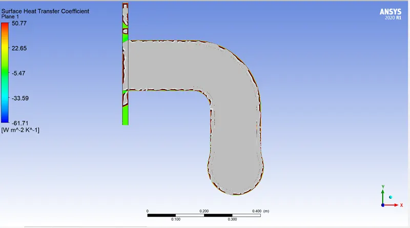
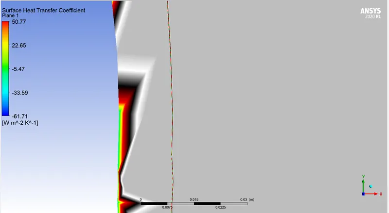
• Heat transfer coefficient:

VALIDATION:

• Reynold's number:

`Re = (rhoxxvxxL) / (mu)`

Where

`rho` = Density = 1.225 kg/m^3.

`v` = Velocity = 5 m/s

`L` = Characteristic length = Diameter of inlet = 170mm

`mu` = Dynamic viscocity = 0.000017894 kg/m.s

The value of Re = 57458.56

• Nusselt number (according to dittus boelter equation):

`Nu = 0.023xx(Re)^(0.8)xx(Pr)^0.33`

For calculating Pr we need the temperature of the fluid inside the convection boundary layer or the film layer

`T_f = (T_o + T_i)/2` = `(700+300)/2 = 500K = 226 C`

Where

`T_f` = Film temperature.

`T_o` = Outer layer temperature = 700K

`T_i` = Inner layer temperature = 300K

• We can round it off to 200C.

Note: If you measure the area weighted average of the fluid and outer convection layer it comes out to be 526K which can be rounded to 500K.

• For 200C, the prandtl value comes out to be 0.698.

From this we can calculate the value of Nusselt number which comes out to be

`Nu = 0.023xx(57458.56)^(0.5)xx(0.698)^(0.3)` = 132.45

We also know that

`Nu = hxxk/L`

Where

• h = surface heat transfer coefficient `W/((m^2K)`
• k = thermal conductivity of air `W/((mK)`
• L = Characteristic length = Diameter of inlet = 0.17 m.

From these values, we can calculate the surface heat transfer coefficient.

`h = (132.45xx0.038)/0.17`= 29.60 `W/((m^2K)`

COMPARISON:

Measured quantitiy	Analytical	Numerical
Surface heat transfer coefficient	21.6 `W/((m^2K)`	29.60 `W/((m^2K)`

CONCLUSION:

• We have performed a steady state pressure based conjugate heat transfer simulation for the exhaust manifold. From baseline meshing, we realised that K-omega SST calculated the values near wall better than the K-Epsilon model. Since, heat transfer near walls had to be calculated K-omega SST proved to be better.
• The outlet of the exhaust had a increased temperature (see temperature plot) because of the increased flow at the outlet. Since, flow volume needed to be conserved the amount of volume flowing through the inlet needed to be equal to the volume of fluid flowing through outlet i.e.,
  • `A_1xxV_1 = A_2xxV_2`
  • Since area is fixed, the velocity needed to be varied which verifies the increased velocity at the outlet.
  • The increased velocity leads to increased temperature at the outlet.
• From the numerical analysis using ANSYS fluent, we determined the surface heat tranfer coefficient for exhaust port which came out to be 18.6 `W/((m^2K)` and through analytical calculation we determined the value to be 29.60 `W/((m^2K)`.
  • With this we realise that the numerical analysis has a error percentage of 27%.