Week 5 - Mid term project - Solving the steady and unsteady 2D heat conduction problem

THIS IS FOR THE STEADY STATE METHOD IN WHICH WE ARE SOLVING THREE METHOD THAT IS JACOBI METHOD,

GAUSS SEIDEL METHOD, SUCCESSIVE OVER RELAXATION

OBJECTIVE:

to solve 2D heat conduction equation by using the point iterative techniques. The Boundary conditions for the problem are as follows;

Top Boundary = 600 K

Bottom Boundary = 900 K

Left Boundary = 400 K

Right Boundary = 800 K

THEORY AND EXPLANATION:

we know the steady-state equation for the steady-state solver

we have a general equation

`(delT)/(delt)+alpha((del^2T)/(delx^2)+(del^2T)/(dely^2)+(del^2T)/(delz^2))=0`

for 2d and the steady-state we eliminate the time term and the we also eliminate the term which varying w.r.t to z that is `(del^2T)/(delz^2`

after that, we get this term`alpha((del^2T)/(delx^2)+(del^2T)/(dely^2))=0`

then we apply the central differencing to the term, then we get

we are applying the central differencing to the term because it his elliptical in nature the ellipticqal term contains the information on the surroundings. so only by means of the central difference, we can getv the information and we can get converge we can get the solution.

`t_(i,j) = alpha((T_(i+1),j-2*T_(i,j)+T_(i-1,j))/(Deltax^2)+(T_(i,j+1)-2*T_(i,j)+T_(i,j-1))/(Deltay^2))`

`T_p =alpha [(T_R-2T_p+T_L)/(Deltax^2)+(T_T-2T_p+T_B)/(Deltay^2)]`

PROGRAMMING:

% 2d heat conduction problem
clear all
close all 
clc

L  = 1;  %LENGTH OF DOMAIN IN METERS
nx = 10;   %number of nodes along xaxis
ny = 10;   %number of nodes along yaxis

%creating the mesh
x = linspace(0,1,nx);
dx= x(2)-x(1);
y = linspace(0,1,ny);
dy= y(2)-y(1);

t = ones(nx,ny); %creating the domain to specifiy boundary condition
%applying the boundary condition
t(1,:)   =  600 ; %temperature at top
t(end,:) =  900 ;%temperature at bottom
t(:,1)   =  400 ;%temperature at left
t(:,end) =  800 ;%temperature at right

%creating the copy of temperatures
t_old = t;

% giving the value for tolerence and error
tol = 1e-4;
error = 9e9;
%defining the value for k as term
term = (dx^2*dy^2)/(2*(dx^2+dy^2));

iterative_solver = input('enter the number for solver method: \n  jacobi=1 \n guauss seidal=2 \n sor=3 \n : ')

  
 if iterative_solver ==1
    %jacobian calculation
    tic
    iter =0;      %incrementing
    while (error>tol)
        for j= 2:ny-1
            for i=2:nx-1
                t(i,j) = term*((t_old(i-1,j)+t_old(i+1,j))/(dx^2)+ (t_old(i,j+1)+t_old(i,j-1))/(dy^2));
            end
        end
        error = max(max(abs(t-t_old)));
        t_old = t
        iter = iter+1;
        
        
    end
time =toc
 end
if iterative_solver ==2
    %jacobian calculation
    tic
   iter =0      %incrementing
    while (error>tol)
        for j= 2:ny-1
            for i=2:nx-1
                t(i,j) = term*((t(i-1,j)+t_old(i+1,j))/(dx^2)+ (t(i,j+1)+t_old(i,j-1))/(dy^2))
            end
        end
        error = max(max(abs(t-t_old)))
        t_old = t
        iter = iter+1;
%         title_text = sprintf('iteration number= %d',iter)
%         title(title_text)
    end
  time = toc
end
if iterative_solver ==3
    %jacobian calculation
    tic
    iter =0      %incrementing
    omega=1.1
    while (error>tol)
        for j= 2:ny-1
            for i=2:nx-1
                t(i,j) = term*((t(i-1,j)+t_old(i+1,j))/(dx^2)+ (t(i,j+1)+t_old(i,j-1))/(dy^2))
                t(i,j) = t_old(i,j)*(1-omega)+(omega*t(i,j));
            end
        end
        error = max(max(abs(t-t_old)))
        t_old = t
        iter = iter+1;
        
    end
    time =toc
end

contourf(x,y,t,'showtext','on')
colorbar
colormap(jet)
title_text = sprintf('number of iterations = %d',iter)
title(title_text)
set(gca,'ydir','reverse')

RESULTS:

this is the plot of the jacobi method figure(1)

we are using the jacobi method for getting the solution of the steady-state equation initially we take the guess value to get the solution. for every iteration, we get the nearly approximate solution as the number of iteration goes on increasing we can get into a better solution. then we get the solution at the particular number of iteration

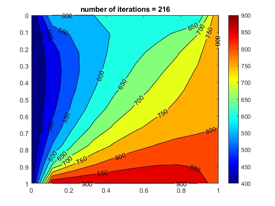
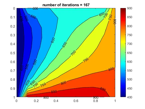
figure 2 is for the gauss seidal method

we are using the gauss seidel method for getting the solution of the steady-state equation initially we take the guess value to get the solution. for every iteration, we get the nearly approximate solution as the number of iteration goes on increasing we can get into a better solution. then we get the solution at the particular number of iteration. but in this method we use the present time step values for the calculation of the temperature at each point

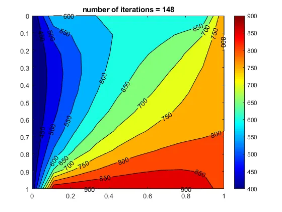
figure(3) is the plot of successive over-relaxation

we are using the successive over-relaxation method for getting the solution of the steady-state equation initially we take the guess value to get the solution. for every iteration, we get the nearly approximate solution as the number of iteration goes on increasing we can get into a better solution. then we get the solution at the particular number of iteration, but we are using the omega and current time step values for calculation of the current time step, as compared to Jacobi and the gauss seidel method we say in less number of iteration we are going to converge.

THIS IS CODE FOR UNSTEADY STATE EXPLICIT SOLVER

OBJECTIVE:to solve the unsteady equation by using the explicit method.

EXPLANATION AND THEORY:

This the equation we get if we want to solve the unsteady state but explicitly we are not using the time marching here .

`(delT)/(delt)=alpha((del^2T)/(delx^2)+(del^2T)/(dely^2))`

for the unsteady term, we are using the forward differencing and for the steady term we are using the central differencing then the term becomes

for the steady term, we used the central differencing because it is elliptical in nature and we get to take the information from the surroundings as all the points are dispersed in the surroundings means the , i say we have to take the information from the boundary sides upper, lower, right, left sides

we are using the forward differencing for the time derivative because we are using the values of temperature as initial values, means for calculation of the next values we take the information from the old values i.e initial values

`(T_(i,j))^(n) =(T_P)^(n-1)+ alpha((T_(i+1),j-2*T_(i,j)+T_(i-1,j))/(Deltax^2)+(T_(i,j+1)-2*T_(i,j)+T_(i,j-1))/(Deltay^2))^n`

then for simple understanding we are using the letter instead on index value

`T_p^(n) =T_P^(n-1) +alpha[(T_R-2T_p+T_L)/(Deltax^2)+(T_T-2T_p+T_B)/(Deltay^2)]^n`

CODE:

clear all
close all
clc
 
 %defining inputs;
 L = 1    % LENGTH OF DOMAIN
 nx = 10 ;   % number of nodes along xaxis
 ny=  10;   %number of nodes along y axis
 dt = 10;
 T= 10000;
 nt = T/dt;
 

 %genearting mesh for number of nodes
 x = linspace(0,L,nx)
 dx = x(2)-x(1)     %defining the mesh size along x axis
 y = linspace(0,L,ny)
 dy = y(2)-y(1)     %defining the mesh size along y axis
 
 %generating the boundary for applying boundary condition 
 %and generating boundary is also the creating the guess values
 t = ones(nx,ny)
 %applying the boundary condition
 t(1,:)= 600
 t(end,:) = 900
 t(:,1) =400
 t(:,end) = 800
 %defining error and tolerence
 tol = 1e-4;
 %creating copy of initial values
 told  = t; %0ld values
 t_prev = t; %previous values
 
 %defining the terms

 alpha =1.4;
 k1 = alpha*dt/dx^2
 k2 = alpha*dt/dy^2
 
 
 

     iter =0;
     for k = 1: nt %time loo
         error=1;
         while(error >tol) %convergence loop
             for j = 2:ny-1  %space loop
                 for i=2:nx-1
                      term1 =1/(1+2*k1+2*k2);
                      term2 = k1*term1;
                      term3 = k2*term1;
                     H = (told(i+1,j)+told(i-1,j));
                     V = (told(i,j+1)+told(i,j-1));
                     t(i,j) =  (told(i,j)*term1)  + ( H*term2) + ( V*term3);

                 end
             end
             error = max(max(abs(t-told)));
             told = t;
             iter = iter+1;
         end
     end



contourf(x,y,t,'showtext','on')
colorbar
colormap(jet)
title_text = sprintf('number of iterations = %d',iter)
title(title_text)
set(gca,'ydir','reverse')

RESULTS:

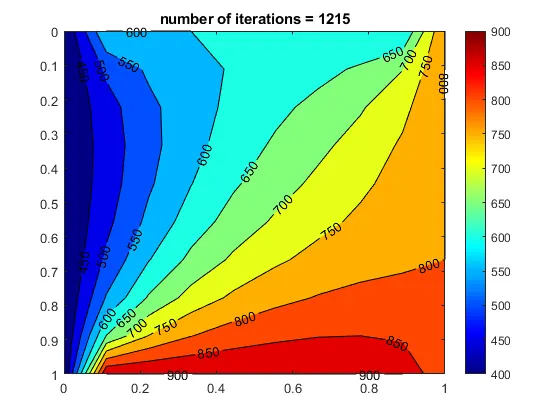
this is the explicit method in this method we are not using the time marching solution but in this method we are usning the ol;d values and we are also not usinhg the iteration met5hod or anyting else by calculatiing the old values and we use old values to calculate the next time step

THIS IS CODE FOR SOLVING THE UNSTEADY EQUATION USING THE IMPLICIT SOLVER:

EXPLANATION AND THEORY:

This the equation we get if we want to solve the unsteady state but explicitly we are not using the time marching here .

`(delT)/(delt)=alpha((del^2T)/(delx^2)+(del^2T)/(dely^2))`

for the unsteady term we are using the backward differencing and for the steady term we are using the central differencing then the term becomes

for the steady term we using the central differencing because it is elliptical in nature and we get to take the information from the surroundings as all the points are dispersed in the surroundings means the , i say we have to take the information from the boundary sides upper, lower , right , left sides

we are using the backward differencing for the time derivative because we are using the values of temperature we we are calculated previously, means for calculation of the next values we take the information from the previous values we have calculated that are previous value i.e initial values

`(T_(i,j))^(n+1) =(T_P)^n+ alpha((T_(i+1),j-2*T_(i,j)+T_(i-1,j))/(Deltax^2)+(T_(i,j+1)-2*T_(i,j)+T_(i,j-1))/(Deltay^2))^(n+1)`

then for simple understanding, we are using the letter instead of on the index value

`T_p^(n+1) =T_P^n +alpha[(T_R-2T_p+T_L)/(Deltax^2)+(T_T-2T_p+T_B)/(Deltay^2)]^(n+1)`

CODE:

clear all
close all
clc
 
 %defining inputs;
 L = 1  ;  % LENGTH OF DOMAIN
 nx = 10 ;   % number of nodes along xaxis
 ny=  10;   %number of nodes along y axis
 dt = 10;
 T= 1000;
 nt = T/dt;
 

 %genearting mesh for number of nodes
 x = linspace(0,L,nx)
 dx = x(2)-x(1)     %defining the mesh size along x axis
 y = linspace(0,L,ny)
 dy = y(2)-y(1)     %defining the mesh size along y axis
 
 %generating the boundary for applying boundary condition 
 %and generating boundary is also the creating the guess values
 t = ones(nx,ny)
 %applying the boundary condition
 t(1,:)= 600;
 t(end,:) = 900;
 t(:,1) =400;
 t(:,end) = 800;
 %defining error and tolerence
 tol = 1e-4;
 %creating copy of initial values
 told  = t; %0ld values
 t_prev = t; %previous values
 
 %defining the terms

 alpha =1.75e-4;
 k1 = alpha*dt/dx^2;
 k2 = alpha*dt/dy^2;
 
 iter_number = input('enter the number for selecting method of iteration: \n jacobi iter \n gauss seidal iter \nsor method\n')
 
 % method 1 that is jacobi method
 if iter_number == 1
    %jacobi method
     iter =0;
     for k = 1: nt %time loo
          error=1;
         while(error >tol) %convergence loop
             for j = 2:ny-1  %space loop
                 for i=2:nx-1
                      term1 =1/(1+2*k1+2*k2);
                      term2 = k1*term1;
                      term3 = k2*term1;
                     H = (told(i+1,j)+told(i-1,j));
                     V = (told(i,j+1)+told(i,j-1));
                     t(i,j) =  (t_prev(i,j)*term1)  + ( H*term2) + ( V*term3);

                 end
             end
             error = max(max(abs(t-told)));
             told = t;
             iter = iter+1;
         end
         t_prev=t;
     end
 end
 

 
 %second method that is gauss seidal method
 if iter_number == 2
    %jacobi method
     iter =1;
     for k = 1: nt %time loo
          error=1;
         while(error >tol) %convergence loop
             for j = 2:ny-1  %space loop
                 for i=2:nx-1
                      term1 =1/(1+2*k1+2*k2);
                      term2 = k1*term1;
                      term3 = k2*term1;
                     H = (told(i+1,j)+t(i-1,j));
                     V = (t(i,j-1)+told(i,j+1));
                     t(i,j) =  (t_prev(i,j)*term1)  + ( H*term2) + ( V*term3);

                 end
             end
             error = max(max(abs(t-told)));
             told = t;
             iter = iter+1;
         end
         t_prev=t;
     end
 end
 

 
 % successive over relaxation method
 
 if iter_number == 3
     %gauss seidal method
      omega = 1.1
      iter =1
     
     for k = 1: nt %time loop
          error=1
         while(error >tol) %convergence loop
             for j = 2:ny-1  %space loop
                 for i=2:nx-1
                     term1 =1/(1+2*k1+2*k2);
                     term2 = k1*term1;
                     term3 = k2*term1;
                     H = (told(i+1,j)+t(i-1,j));
                     V = (told(i,j+1)+t(i,j-1));
                     t(i,j) =  (t_prev(i,j)*term1)  + ( H*term2) + ( V*term3);
                     t(i,j) = told(i,j)*(1-omega)  + omega*t(i,j);

                 end
             end
             error = max(max(abs(t-told)))
             told = t;
             iter = iter+1;
         end
         t_prev=t
     end
 end
 contourf(x,y,t,'showtext','on' )
 colorbar
 colormap(jet)
 title_text= sprintf('number of iteration = %d',iter)
 title(title_text)
 set(gca,'ydir','reverse')

RESULTS:

this is the plot of the Jacobi method figure(1)

we are using the jacobi method for getting the solution of the steady-state equation initially we take the guess value to get the solution. for every iteration, we get the nearly approximate solution as the number of iteration goes on increasing we can get into a better solution. then we get the solution at the particular number of iteration

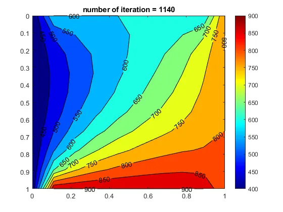
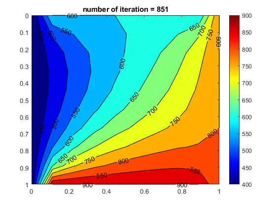
figure 2 is for the gauss seidel method

we are using the gauss seidel method for getting the solution of the steady-state equation initially we take the guess value to get the solution. for every iteration, we get the nearly approximate solution as the number of iteration goes on increasing we can get into a better solution. then we get the solution at the particular number of iteration. but in this method we use the present time step values for the calculation of the temperature at each point.we do same procedure and we use the time mar4ching solution here so we add the time loop here .

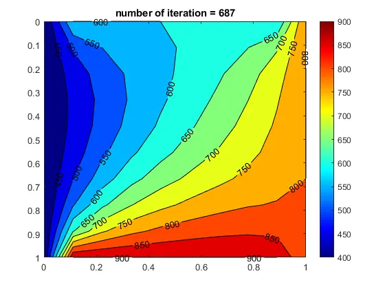
figure(3) is the plot of successive over-relaxation

we are using the successive over-relaxation method for getting the solution of the steady-state equation initially we take the guess value to get the solution. for every iteration, we get the nearly approximate solution as the number of iteration goes on increasing we can get into a better solution. then we get the solution at the particular number of iteration, but we are using the omega and current time step values for calculation of the current time step, as compared to Jacobi and the gauss seidel method we say in less number of iteration we are going to converge. we do same procedure and we use the time mar4ching solution here so we add the time loop here .

CONCLUSION:

by solving this problem i get to know the how to solve the boundary condition problem using the matlab and also know what are steady terms and the unsteady terms in the equation and how to solve them using the different methods iof the iterrations.