Week 3 - External flow simulation over an Ahmed body.

AIM: to simulate the flow of the air through the Ahmed body and providing the correct results

describing the importance of the Ahmed body

explaining the negative pressure in the wake region

DESCRIBING THE IMPORTANCE OF THE AHMED BODY:

1. Ahmed Body and Its Importance:- Ahmed body is a simplified car body and was first created by S.R Ahmed.This shape provides a model to study geometrical effects on the wakes of ground vehicles. This is the kind of baseline geometry for automobile bodies. The flow of air around Ahemd body captures the essential flow features around an automobile and it describes how to calculate the turbulent flow field around a simple car-loke geometry using the turbulent, flow, K-epsilon interface. People working in vehicle aerodyanamics use Ahemdbody to validate their numerical model because the experimental data for Ahemd body. Once the numerical model is validated, its is used to design new models of the car and also used for faster calculation and for comparision of analytical results.

Geometry of Ahem-body

significance of ahmd body

• ahmd body is the simplest model of car we are simulatin or doing the simulation on that because of the we want to study how the velocity and flow of the air which id going to effect the body of the car.
• if we know the how the flow going to effect the drag co efficient and the lift co efficient for the simplest geometry. than for the complex shapes we can understand how if going to effect on the shape.
• why they are doing the testing on the ahmd body because the collection of data like pressure velocity and some other properties in simplest model is easy. and we can compare it with a complex shapes .

EXPLAINING ABOUT THE NEGATIVE PRESSURE In THE WAKE RE3GION:

we know the ciontinuity equation

`rho_1a_1v_1= rho_2a_2v_2`

• this equation givew us the relation between the law of conservation of the mass flow rate . i.e mass flow rate is conserved in thye both side of the pipe. i.e inlet is equal to the outlet .
• assume the velocity and area are changing but the density of the flow remains constant .
• because the we are assuming it as the in compressible flow>

then equation becomes

`a_1v_1=a_2 v_2`

a is the area

v is the velocity

• if a1 >a2 the v2>v1.
• if a2>a1 then v1>v2.

now we come to bernoulis equation in terms of the head

`(p_1/(rhog)+(v_1^2)/(2*g)+z_1)=(p_2/(rhog)+(v_2^2)/(2*g)+z_2+h_g)`

where

p1, p2 are the pressures the the section 1 and section 2

v1, v2 are the velocities at the section 1 and section2

z1 ansd z2 are the head

hg is the frictional losses

• assume that the head difference is equal z1 and z2 get canceled
• by this we can say if area increases pressure iincreases.
• and if the area decreases the pressure decreases.

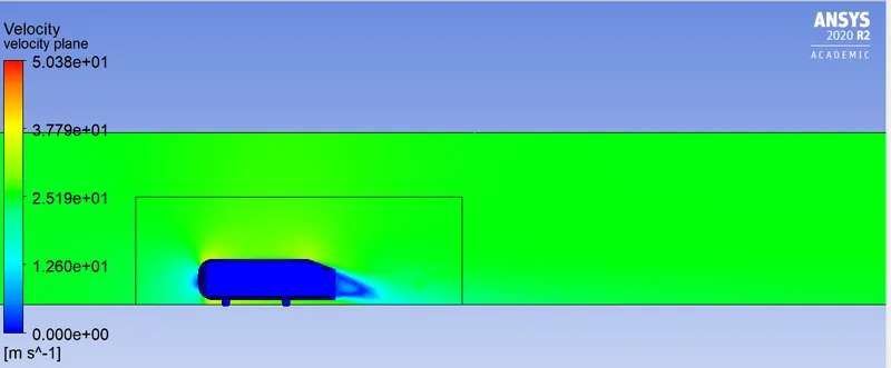
velocity contour:

this contours showing the velocity and the pressure how they are changing with the increase in he velocity and pressure.

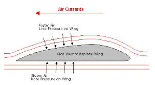
IF WE WANT TO UNDERSTAND WHY PRESSURE IS LESS IN THE WAKE REGION WE HAVE TO UNDERSTAND THIS FIGURE

• this upper and lower stream lines showing the movement of layers of the air >
• in the upper side, the area is large and velocity is high. and pressure is low.
• upper stream lines (fluid in the upper side has to travel a longer distance at the same time. so it creates the low-pressure region.
• this makes the lower region to creates high pressure i.e enormous amount of pressure is created in the lower region that lifts the planes.

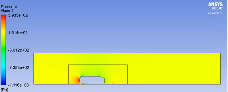
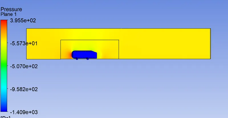
pressure contour:

velocity contour

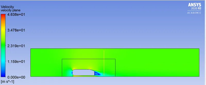
• at the centre leading end the velocity is zero and the pressure is very high that point we called as the stagnation point.
• as the air starts to flow on the upper region it will stick to the surface of the ahmd body and velocity is very low at the points.
• as it goes to the railing end the suddenly increase in the area seperates the air from the surface of the ahmd body and velocity is very low and creates the vaccum in the area i.e negative pressure.
• the pressure diffrence between the atmosphere and the wake area is very high.

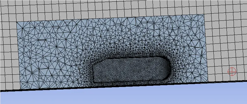
MESH INDEPENDENCE TEST( GRID INDEPENDENCE TEST):

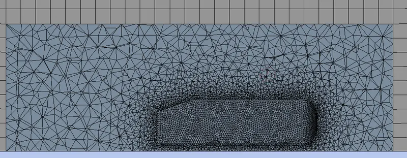
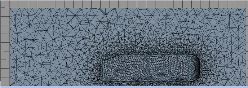
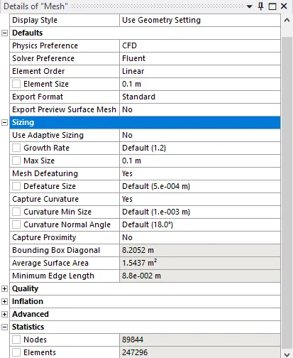
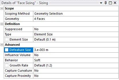
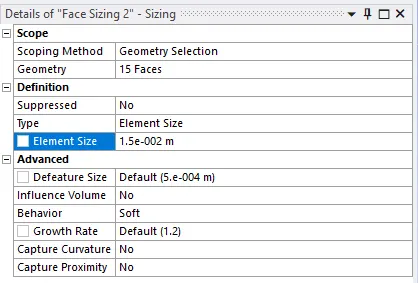
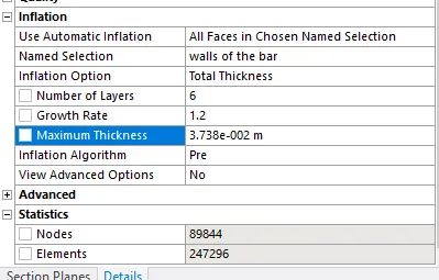
CASES	CASE 1	CASE 2	CASE 3
number of elements	247296	255321	451131
element size for face of the ahmed body	0.015m	0.018m	0.013m
total thickness of inflation layer	0.03738m	0.006460m	0.0014229m

MODELLING APPROACH:

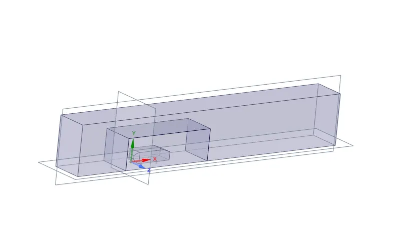
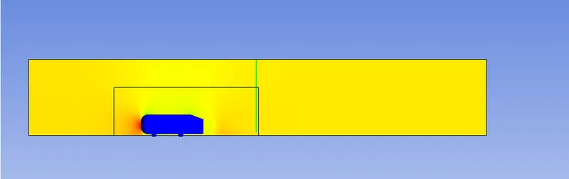
• to perform the simulation we have to produce the produce the correct enclosure to the ahmed body first.
• so we use th sapce claim to do so.
• we create the two enclosures one enclosure for the wind tunnel.
• another enclosure for the mesh grading
• we on the interferences for the to flow the physics correctly.

MESH:

• for the mesh of the we have chosen the hexahedral mesh because that mesh gave us the best results.
• for the first enclose we have chosen the tetra mesh which has the more cpacity to capturte the curvature.
• in the circular region below the ahmd body i.e at its legs we have cteated the inflation layers.
• to capture physics perfectly .
• and for surface of the ahmed body we crteated the mesh with smaller elements.

SOLVER REQUIRE MENTS OR SOLUTION:

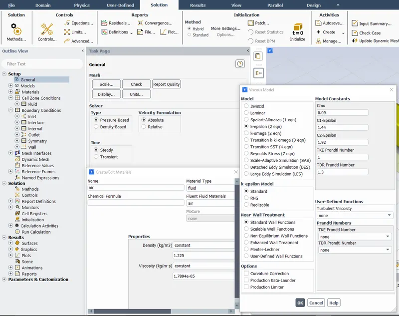
• in this solution we are not using the energy equation because we are not solving for the temperature.
• we are using the pressure based solver because our mach number is below 1.
• we use the simple sover because the velocity and pressure are not coupled.
• for the selection of the material we use air as the flow material.
• in the refrence values we specify the area and length of the domain.
• we apply boundary conditions for the problem what according tyo the problem.
• we create the reports in the definition option.
• we create the contours in the contour options .
• we use hybrid initialization for the problem.

RESULTS:

• we use the cfd post for the post processing of the results.
• after that we create the planes and the for looking at the velocity contours and the pressure contours.

RESULTS:

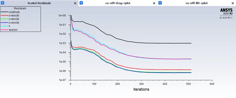
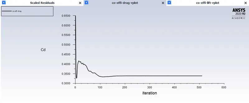
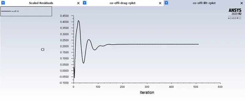
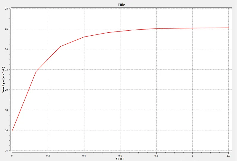
CASE1

RESULTS FOR THE CASE 2

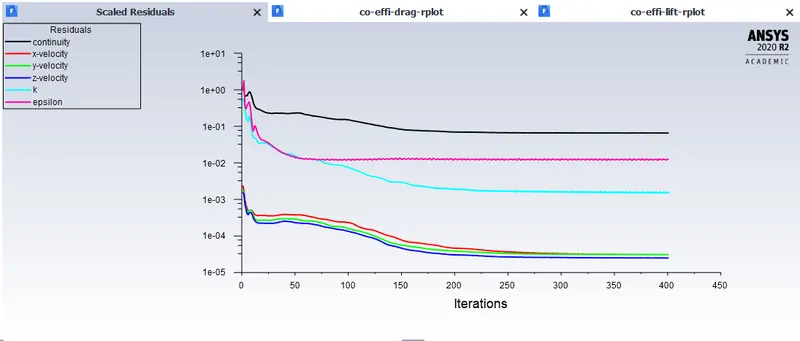
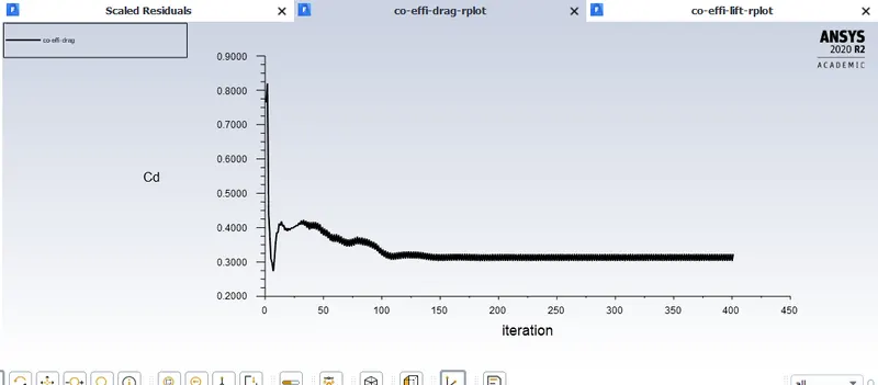
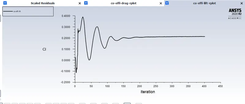
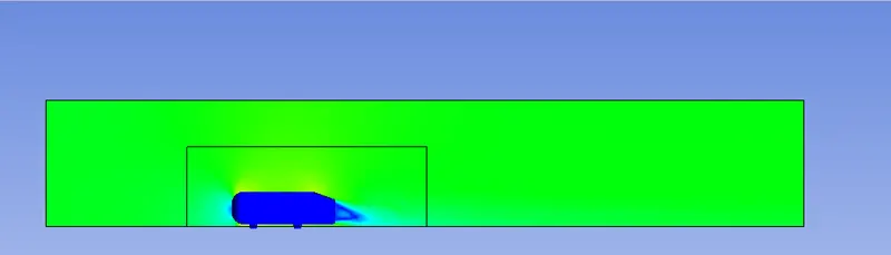
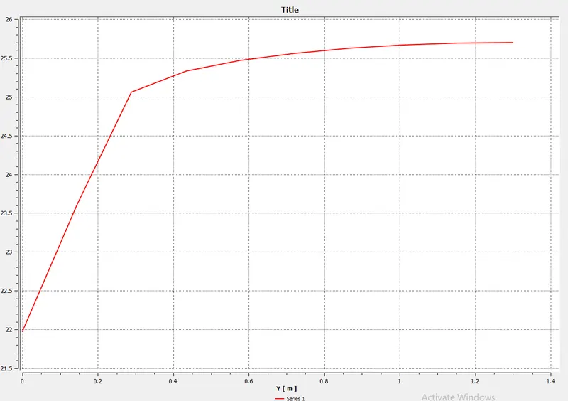
RESULTS FOR THE CASE THREE:

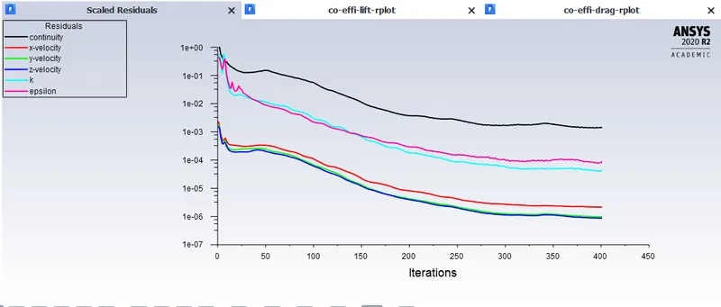
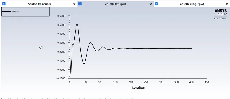
list of results for different mesh sizes

CASES	CASE1	CASE2	CASE3
drag coefficient	0.3388	0.3231	0.3279
lift co efficient	0.2162	0.2105	0.2348