Week 3 - Solving second order ODEs

OBJECTIVE:

To describe the transient behavior of a system i.e simp pendulum.

objective is to write a program that solves the following ODE. This ODE represents the equation of motion of a simple pendulum with damping.

EQUATION:

`(d^2(theta))/dt+b/m(d(theta))/dt+g/l*sintheta=0``

by breaking down second order ode's into number of first order ode"s we ge3t this equation.

`(d(theta)_1)/dt+(b(theta)_2)/m+g/l*sintheta=0`

`(d(theta))/dt=theta_2`

b=damping co_efficient.

g= acceleratiopn due to gravity i.e 9.8 m/s.

l= length of the wire in which pendulum is hanging.

m=masss of the pendulum.

PROGR0MMING LOGIC:

1. by using input comman we assign the value to damping, accelerationn due to gravity,length,mass.

2.Theta_0=[0;5]theta_0 is an array which carrying the values of displacements and angular velocity i.e displacement and angular velocity.

3.linspace(0,20,500) we are using the linspace here because we need plot the distanve and velocity in 500 values.from interval 0-10 seconds.

4.ode45 we are calling subcalling function here and using the ode45 solver to solve the given diffrential equation heretheta refers to the ode45 where t is time interval and theta refer to the value of angular velocity and displacement.

5.plot comment used to plot the results then we are plotting (t,results) vs all row value values of angular velocity that is colum in matrix.

6.subplots are used to plot 2 plots in a single figure in which(x,y,z) x, y indicates the rows and columns to be added and z indicates the position of the graph where youn want to plot.

7. legend command is used to name the graph .

9.hold on we are using the hold on commennt to over lap the tow diffrent curves of angular velocity and displacemenplot comment used to plot the results then we are plotting (t,results) vs all row value values of displacements and single column in matrix.

10.hold off is used to stop the over lapping.

11.we are labelling the x -axis as the plot using plot commandxlabel('time')

12.we are labelling the y -axis as the time using the plot command.

13.we are calling the sub function here and defining the values of the damping acceleration due to gravity,length of pendulum, mass.

14.dtheta1_dt=theta(2); we applying the deffrential equation here the theta(2),it calculate the value od another difrentialm equation , then is send the value of angular velocity and displacement to primary equation and so on untill the intervals run ot.

15.theta2_dt=-(b/m)*theta(2)-(g/l)*sin(theta(1)) this equation we genrate from given 2nd order diffrential equation dtheta_dt=[dtheta1_dt;dtheta2_dtwe are defining the comined diffrential array of angular velocity and displacements.

16.axis command is used to fix the axis at the ficed poin.

17.pause is used to plase the video for certain time .

18. movie command is used to generate the movie of the given file.

19.video writer used to save the file as avi.

20.video writer used to save the file as avi.

CODE :

close all 
clear all
clc
%INPUTS
b=0.05;                                                   % by using input comman we assign the value to damping, accelerationn due to gravity,length,mass.
g=9.8;
l=1;
m=1;


%initial input

theta_0=[0;3]                              %theta_0 is an array which carrying the values of displacements and angular velocity i.e  displacement and angular velocity.
%time_period

t_span=linspace(0,20,500);                %  we are using the linspace here because we need plot the distanve and velocity in 500 values.from interval 0-10 seconds.


%solve ode

[t,results]=ode45(@(t,theta)ode_func(t,theta,b,g,l,m),t_span,theta_0); %we are calling subcalling function here and using the ode45 solver to solve the given diffrential equation here
figure(1)
subplot(2,1,1)
plot(t,results(:,1));                              %t,theta refers to the ode45 where t is time interval and theta refer to the value of angular velocity and displacement
hold on;                                           %we are using the hold on commennt to over lap the tow diffrent curves of angular velocity and displacement 
plot(t,results(:,2));
legend('Ang. Displacement','Ang. Velocity')           % legend command is used to name the graph.
xlabel('time (s)')
ylabel('Amplitude')
title('Variation of Ang disp and Ang vel with time')
hold off;                                              % hold off is used to stop the over lapping



subplot(2,1,2)                                 %subplots are used to plot 2 plots in a single figure in which(x,y,z) x, y indicates the rows and columns to be added and z indicates the position of the graph where youn want to plot
plot(results(:,1),results(:,2));
xlabel('position-radians');                     % we are labelling the x -axis as the plot using plot command
ylabel('angular velocity');                     % we are labelling the y -axis as the plot using time command
 

ct=1
 
figure(2)
for i=1:500
    x0=0;
    y0=0;
    x1=1*sin(results(i,1));
    y1=-1*cos(results(i,1));
    
      plot([x0,x1],[y0,y1])
   hold on
     
     plot(x0,y0,'marker','square','markersize',25,'markerfacecolor','b');
     plot(x1,y1,'marker','o','markersize',15,'markerfacecolor','w');
    
   
    
   
     
   
    hold off;
    axis([-1.5 1.5 -1.5 0.5]) %axis command is used  to fix the axis at the ficed poin.
    
    
    
    M(ct)=getframe(gcf)
    ct=ct+1;
    pause(0.05) % pause is used to plase the video for certain time  .
    
    
        
                    
end
movie(M)             % movie command is used to generate the movie of the given file 
videofile=VideoWriter('pendulum.avi','uncompressed AVI'); % video writer used to save the file as avi.
open(videofile)       %open  command is used to open the video file which we have created using the command.
write(videofile,M) 
close(videofile)

SUB CALLING PROGRAMME:

function[dtheta_dt]=ode_func(t,theta,b,g,l,m) %we are calling the sub function here and defining the values of the damping acceleration due to gravity,length of pendulum, mass


dtheta1_dt=theta(2);   % we applying the defential equation here  the theta(2),it calculate the value od another difrentialm equation , then is send the value of angular velocity and displacement to primary equation and so on untill the intervals run ot.

dtheta2_dt=-(b/m)*theta(2)-(g/l)*sin(theta(1)); %  this equation we genrate from given 2nd order diffrential equation 

dtheta_dt=[dtheta1_dt;dtheta2_dt]; %we are  defining the comined diffrential array of angular velocity and displacements. 

end

RESULT :

this figure showing the relation between the tinme versus the displacement and the angular velocity. this relation genrate the graph which show how the waveas are genarated for particular value of velocity.

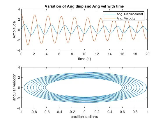
this vide3o shows the animation the simple pendulum which is done by the matlab using the python language.

CONCLUSION:

after attendind this session we are able to generate the animation of the simple pendulum . we know the theoriies abot the simple pendulum , and we know how to solve the second ordeer ode's using the matlab ,we le learn how the angular veloccty and displacement is relating to each other.