Week 2 - Flow over a Cylinder.

AIM : to simulate the flow over the cylinder by using the steady-state solver and unsteady state solver and explaining the phenomenon of Karman vortex shedding.

part1 : to simulate the flow using the steady-state and unsteady state solver.

introduction to the flow over a cylinder:

2. Unsteady state flow around a circular cylinder immersed in a
uniform flow
The following Navier-Stokes equation of the motion of fluid with incompressible viscous flow is
used; this equation indicates that the inertia force, pressure, and viscous force are in equilibrium.

`rho (Du)/(Dt) = -gradp + mu Deltau`

[inertia force] [pressure] [viscous force]
where ρ is the density, u is the velocity vector, t is the time, p is the pressure, and µ is the
coefficient of the viscosity.
Fluid flow analysis aims to determine the relationship between pressure and flow velocity by
solving Equation 1, which is subject to a geometric boundary condition, i.e., the interface surface
at which a fluid contacts a solid object. As very small uneven roughness is unavoidably distributed
over the whole surface of a solid object, fluid particles are completely captured on the solid
surface due to the viscosity of the fluid. This property of fluids leads to a very important
assumption such that a condition of zero fluid velocity (i.e., no slip) is achieved over the whole
surface of a solid object.
The relative importance of the ratio of the inertial forces to the viscous forces for the flow
conditions is quantified by taking L as the characteristic scale of flow and U as characteristic
velocity of flow; D Dt ≈ L U , 2 ∆ ≈1 L can then be introduced, and the index yields:

`R_e = (rho vl)/mu`

where Re represents a dimensionless number called the Reynolds number. If the Navier-Stokes
Equation 1 is converted to a dimensionless form, it is well known that this dimensionless equation
depends on only the Reynolds number. Thus, if Reynolds numbers are identical, an overall field
containing every individual flow with a geometrically similar boundary shape to each other can be
regarded as being similar overall. In addition to increasing velocity, a greater density, a smaller
viscosity, or a larger solid body size tend to increase the Reynolds number, thereby equally
affecting the overall flow field. Accordingly, it can be said that the Reynolds number represents a
dimensionless flow velocity.

Flow patterns generated around a circular cylinder immersed in a uniform flow are shown in
Figure 1 (Hughes & Brighton, 1999). In relation to the flow around an object, a combination of a
uniform flow with a circular cylinder will be the simplest case. The pattern of this flow varies
depending upon the Reynolds number.

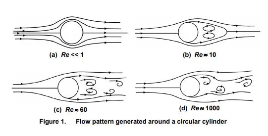
Figure 1-(a) shows a flow with a very small Reynolds number. The shape of every streamline is
symmetrical not only around the cylinder’s upper to lower side, but also around its front to rear.
As the Reynolds number increases, the front to rear symmetry disappears, and the interval of the
streamlines of the cylinder’s rear flow widens. As the Reynolds number reaches close to 10, a
closed region of the streamline is generated within the cylinder’s rear flow. The fluid in the upper
half of this region rotates clockwise, and the fluid in the lower half rotates counterclockwise. This
phenomenon is the result of the so-called generation of vortices. Figure 1-(b) depicts this state.
As the Reynolds number increases, the length of the vortex increases. When the Reynolds number
exceeds 60, the rear flow becomes unstable as shown in Figure 1-(c), and the vortex begins to
oscillate in an up-down direction. The fully formed vortex is carried away on the surrounding
main flow, and a vortex subsequently occurs on the other side. This vortex then expands before
finally dissipating and departing leaving the circular cylinder. In addition to this flow process,
every pair of upper and lower vortices behind the cylinder is stored in an alternative regular array
to form twin rows of vortices. These rows are called the von Karman vortex street. While the main
flow approaching the circular cylinder is in a uniformly steady state, a periodically varying flow
characteristic of the von Karman vortex street appears in the cylinder’s rear flow.
As shown in Figure 1-(d), as the Reynolds number reaches 1,000, the vortices are mixed together,
and the flow behind the cylinder (wake) behaves very irregularly in time and space scale. This
behavior is the so-called state of turbulent flow. However, a free stream distant from the wake
region maintains a steady state, and the streamlines are held in a regular and smooth shape. This
phenomenon is known as laminar flow.
Abaqus/CFD was used in this study to perform analyses, within a range of Reynolds numbers up
to 200 under which we considered it possible to analyze the occurrence of laminar flows.

EFFECT O FTHE REYNOLDS NUMBER OUON THE COEFFICIENT OF DRAG DRAG :

as the reynolds number increases, the velocity increases the velocity increase means we know the formula for drag

`F_(drag = (c_d rhoAv^2)/2`

DRAG FORCE depends upon the square of the velocity as the velocity increases drag force also increase,

so we can say that the as reynolds number i9ncreases the drag force also increases.

BUT WE WANT THE RELATION WITH CO-EFFICIENT OF DRAG

`C_d = F_(drag)/(rhoAv^2`

as the velocity increases the so the co-efficient of drag depends upon the inversely proportional to the velocity square. so we say that as velocity increases the co-efficient of drag decreases

MODELLING APPROACH:

geometry

• for modelling the approach we are starting with the creation of geometry . first we get into the geometry section where we create the geometry using the space claim.
• first we select the unit in meters as required dimensions are given we create the geometry using the tools .
• we remove the extra edges using the deleting construction lines.
• we use pull command to make it a surface .
• and we remove the circular area to create the cylinder .

meshing

• we use a meshing tool to mesh the geometry.

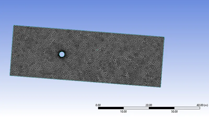
• first we create the mesh by giving the element size i.e 0.27 meters.
• and we convert the quad dominated mesah into triangle dominated mesh
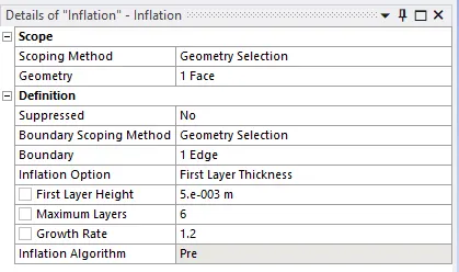
• we have to capture the physics at the circumference of the cylinder is perfectly so we divide circle into 36 parts .
• and then to create body fitted mesh we are adding the inflation layers to capture the physics more clearly.
• if we are not getting the correct results for this element size , again we change the mesh size to capture solution corretly.
• after meshing we create the named selections of boundary.
• we gave the name to each of the faces of the boundaries.

setup

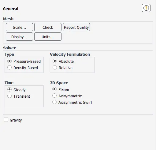
• we are using the pressure based solver because the mach number is less then 0.8.
• and steady-state because are not solving the time derivative .
• we only solve time derivate when we want time-accurate solution . how may quantities are changing according to the time.

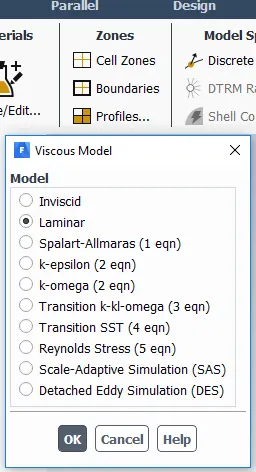
• we are using the viscous laminar moldel because flow is laminar reynoldws number is less.
• we create the user defined material which has viscocity of 0.05 m^2/s and density of 1kg/m^3 because we have to see how vortex shedding is happening.
• then we apply the required boundary conditions as the problem .

• then we create the plots or reports using the option definitions as the required plots we want
• we are using the hybrid initialization because the initials guess values are taking according to the solver.

solution

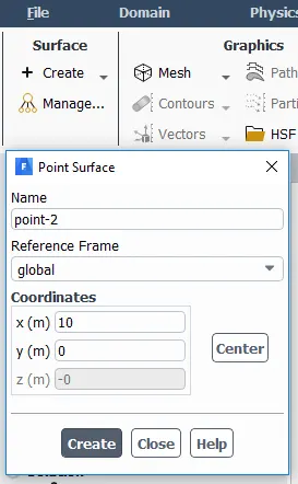
• for getting the graph of the vortex veocity we greated the monitor ppoint using the create >points > at a distance of 10 meter we create point you can give any name to the point.
• and we can get to now about the distance there vortex shedding happening is by trail and error method

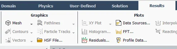
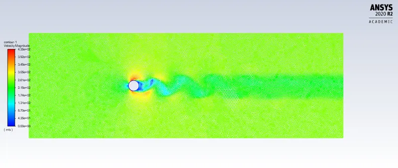
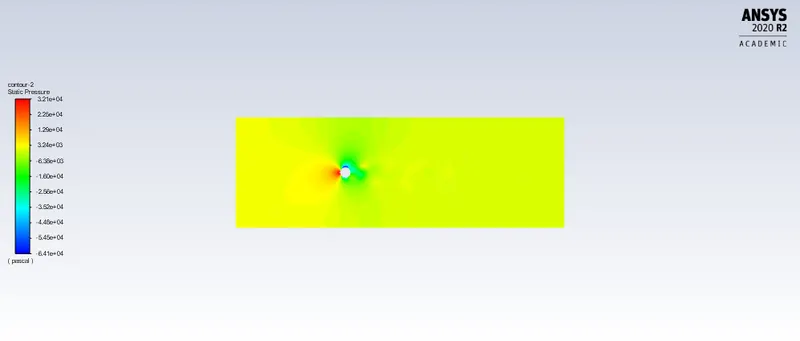
• we can create contours of the velocity and the pressure using the contour option.

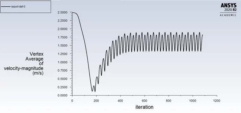
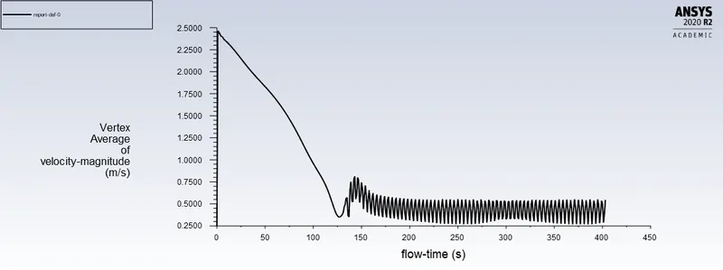
calculation of strohul number for transient state solution for reynold's number is equal to 100

`st = (omega*L)/u`

`omega`= frequency of vortex shedding

L= charecterstics length

u = velocity of the fluid

`st = (0.27*2)/2.5`

st =0.216 Hz

PRESULTS :

GRID INDEPENDENCE TEST:

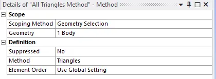
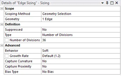
• grid independence is the test where we took the results for different sizes of mesh. and we select the optimum mesh means course mesh than other which gave us the same results . in other words the further decrease in the element size dosent effect the solution because the error is very small.
• so we choose the mesh which gave us the same result, but has a bigger element size to reduce the computational time.

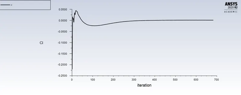
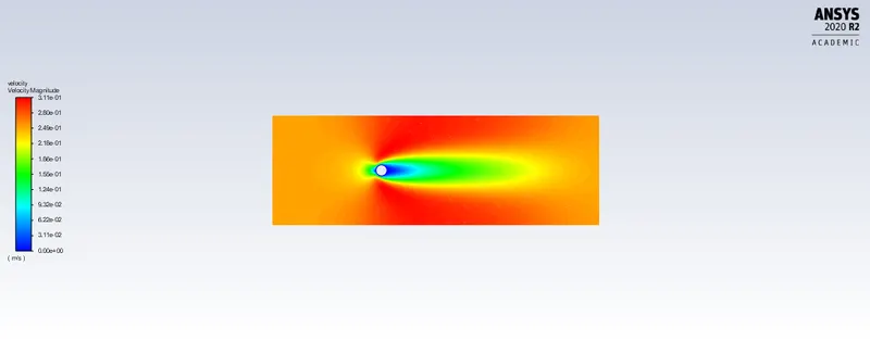
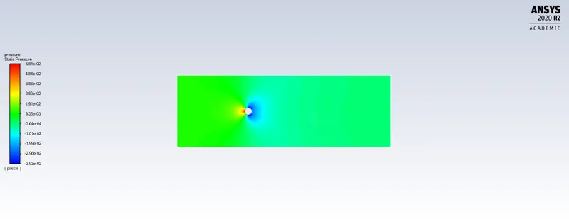
RESULTS FOR THE REYNOLDS NUMBER 10

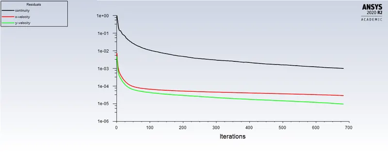
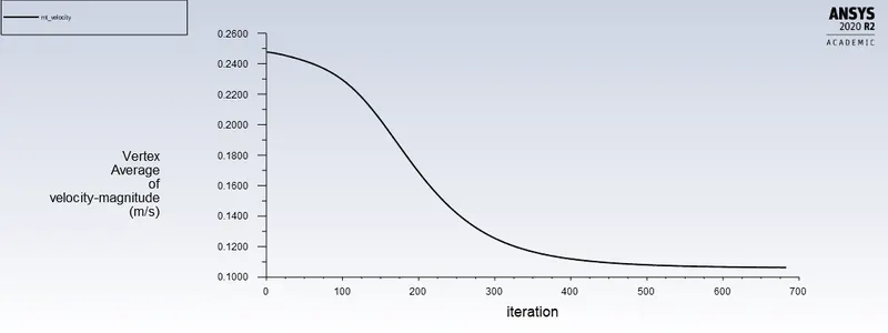
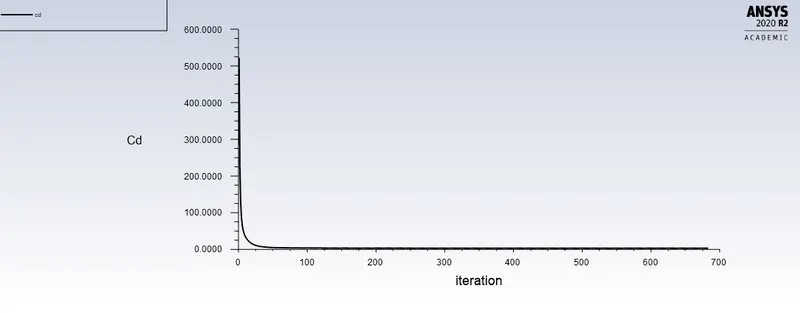
RESULTS WHEN THE RENOLDS NUMBER ARE IS 100

RESULTS FOR REYNOLDS NUMBER 1000:

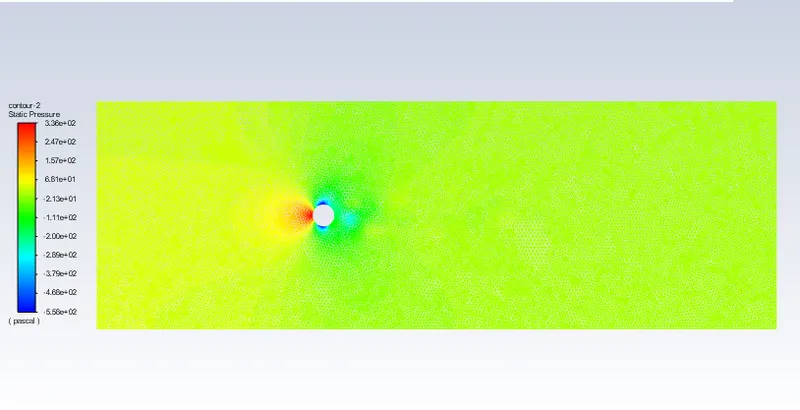
RESULTS FOR THE REYNOLDS NUMBER 10000

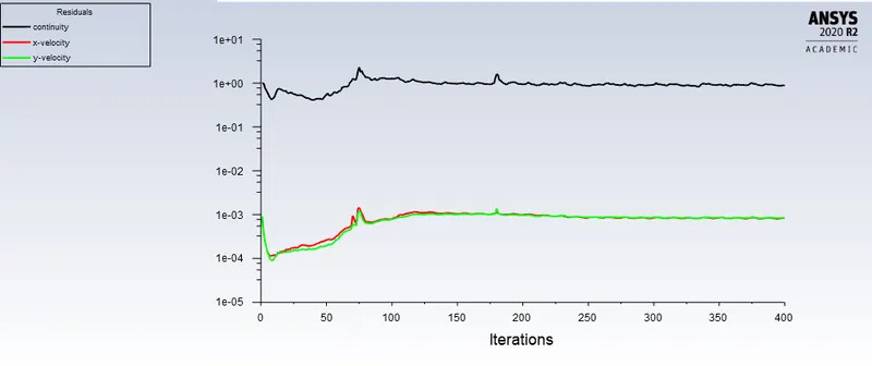
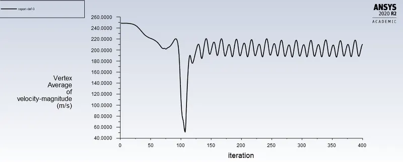
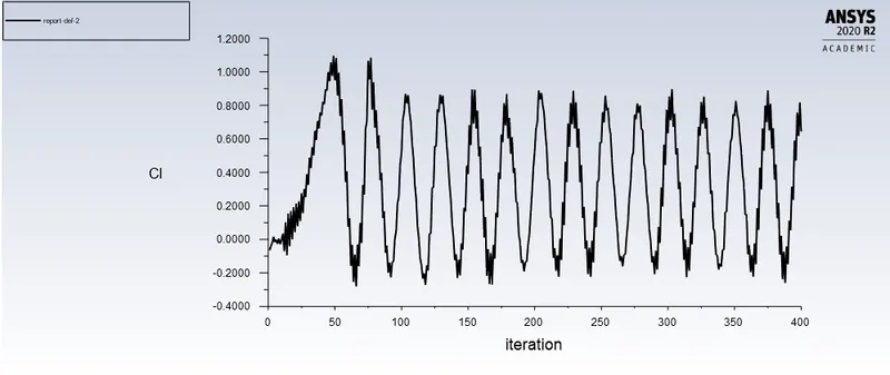
RESULTS FOR REYNOLDS NUMBER 100000:

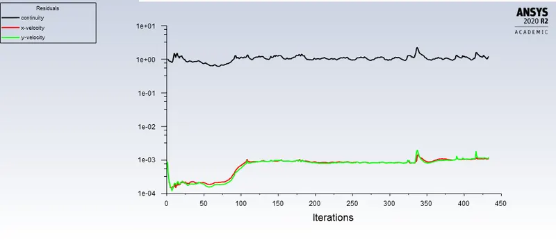
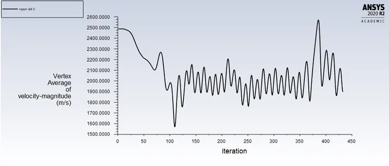
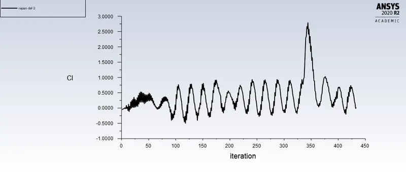
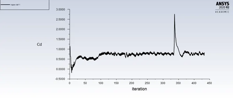
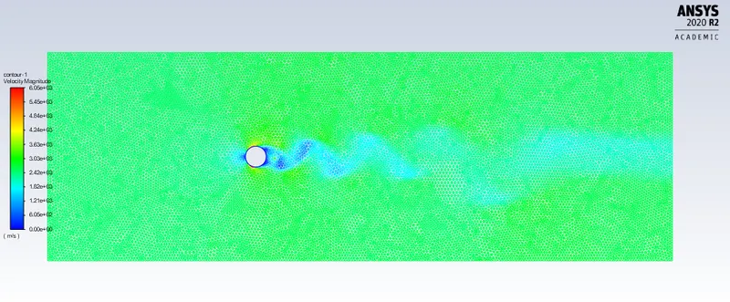
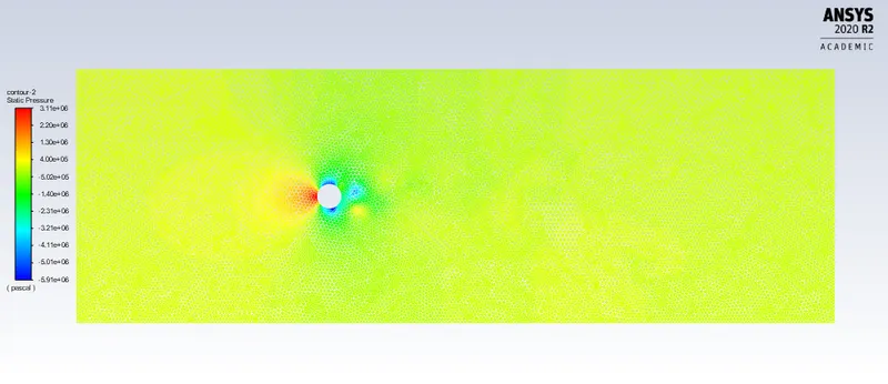
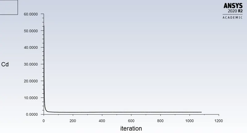
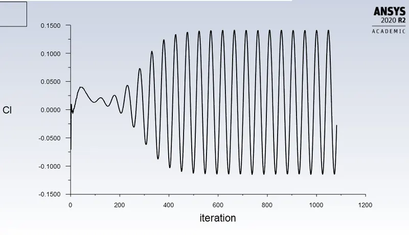
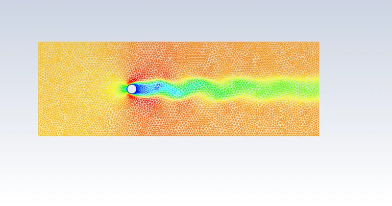
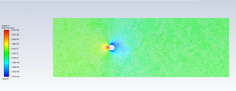
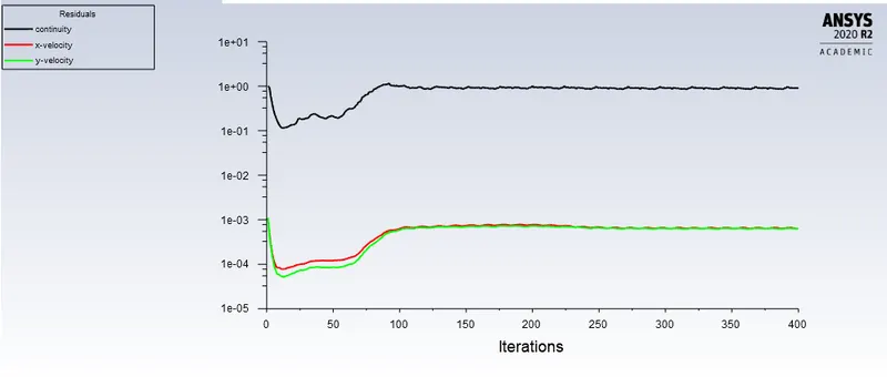
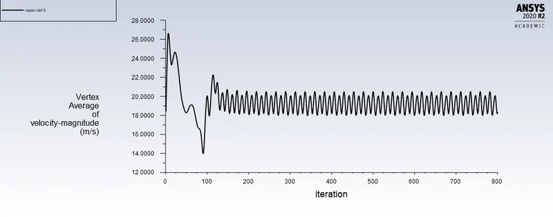
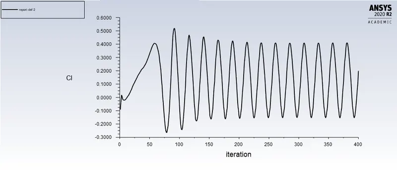
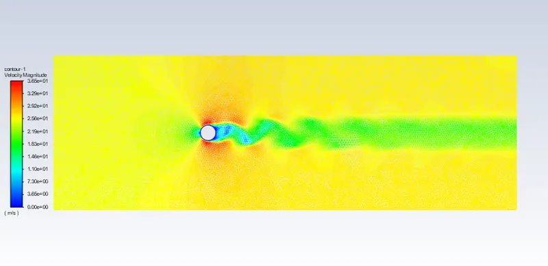
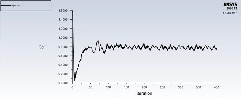
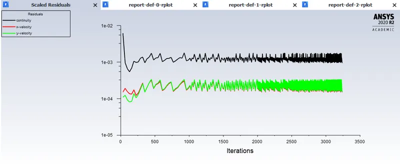
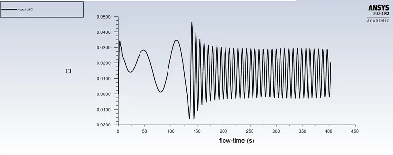
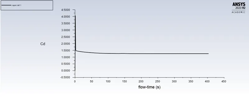
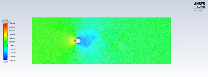
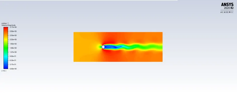
RESULTS FOR REYNOLDS NUMBER 100 WITH TRASIENT SOLVER :

THE CURVE SHOWS THE VARIATION OF THE CO-EFFICIENT OF DRAF WITH INCREASE IN THE VALUE OF THE VELOCITY

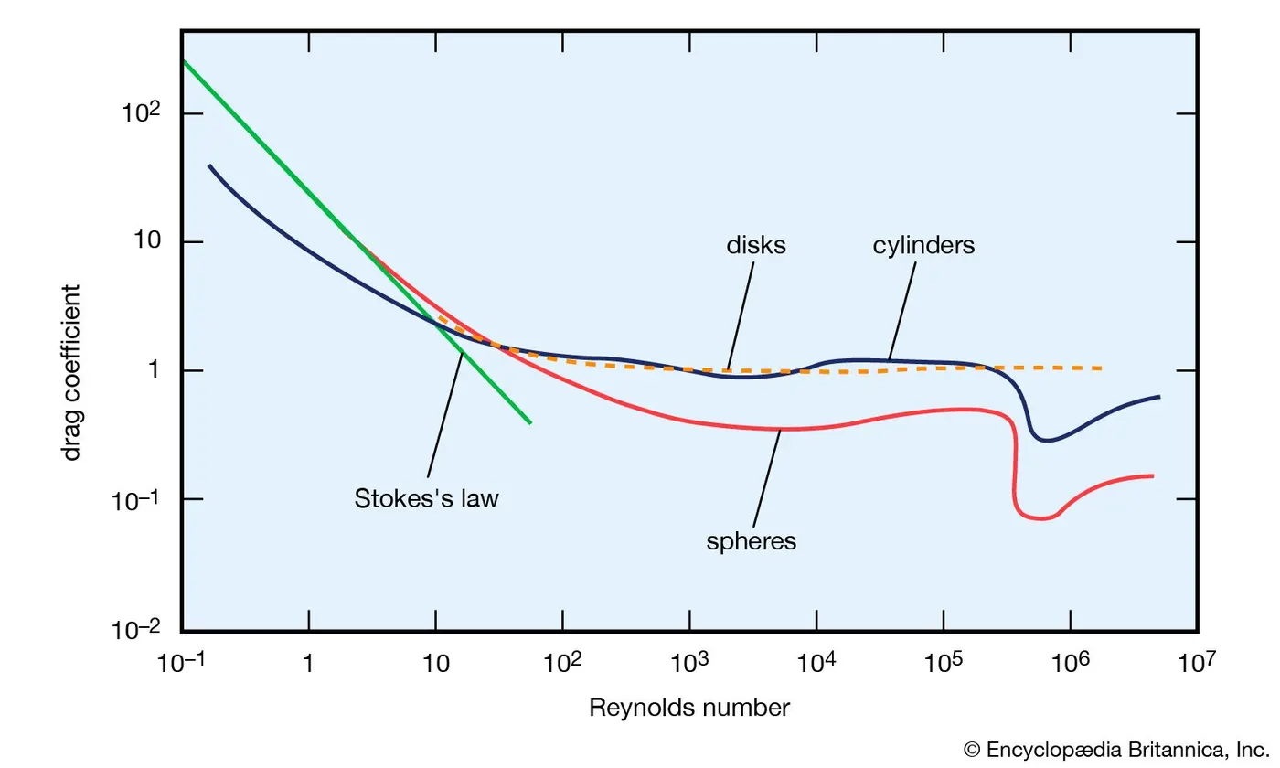
• this graph showing the variation of the c o-efficient of the drag with them variation of the Reynolds number
• as the Reynolds number increases the we know the velocity increases cd is inversely proportional to the velocity so cd decreases cd(co efficient of drag)

RESULTS FOR TRANSIENT SOLVERS :

CASES	SOLVER	DRAG CO-EFFICIENT	LIFT CO-EFFICIENT
REYNOLD NUMBER =10	STEADY STATE	3.33	0.009658
REYNOLD NUMBER =100	STEADY STATE	1.3	0.01372
REYNOLD NUMBER =1000	STEADY STATE	0.721	0.204
REYNOLD NUMBER =10000	STEADY STATE	0.705	-0.270
REYNOLD NUMBER =100000	STEADY STATE	0.682	-0.335
REYNOLD NUMBER =100	TRANSIENT STATE	1.2379	0.0138

https://www.sciencedirect.com/science/article/pii/S0307904X08000243