Week 9 - FVM Literature Review

DIFFERENCE BETWEEN FDM AND FDM

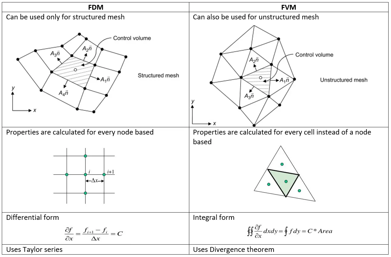
2. Differences between Finite Volume Method and Finite Difference Method

		Finite Volume Method (FVM)	Finite Difference Method (FDM)
1.	Grid Generation	Domain is divided into control volumes or cells with variable of interest located at the centroid of each control volume.	Domain is divided into points with each point representing variable of interest.(that are grid points)
2.	Discretization	Differential form of governing equations are integrated over each control volume i.e., discretization is based on fluxes.	Differential form of governing equations are replaced by system of algebraic equations at each grid point, or in other words, discretization is based on derivatives.
3.	Laws of conservation	Conservation principles including mass, momentum and energy are maintained by definition.	Conservation laws are not preserved in all cases.
4.	Applicability	Structured and unstructured grids as shape of control volume does not impact conservation principles.	Structured grids in most cases.
5.	Examples of Numerical Schemes	Upwind Differencing, Hybrid Differencing, Power Law : Convection-Diffusion problems	Forward difference, backward difference, central difference
6.	Advantages	Robust in terms of performance with respect to challenging problems that cover both academia and industrial physical processes, cheap in regards to quick and reliable coding.	Easier implementation, availability of higher order schemes, and generally lower computational cost and improved efficiency over FVM for problems of similar nature with simpler grid structures.
7.	Disadvantages	Presence of false diffusion when lower order accuracy upwind schemes are preferred due to stability issues in higher order accurate schemes like central differencing, and difficulty to accomplish higher order schemes in comparison to FDM.	Use of mapping functions in methods like variable transformation technique is required when point(s) are not aligned along cartesian coordinates which becomes increasingly challenging with more complex geometrical features.
8.	Applications	Physical Problems: Evaluation of external aerodynamics features of aircraft bodies, analysis of different heat transfer modes and mechanisms when graphics processing unit (GPU) on a graphics card dissipates power within an enclosed domain, assessment of wells in petroleum engineering. Commercial Softwares: ANSYS CFX, ANSYS FLUENT, PHOENICS, STAR-CD, OpenFOAM	Physical Problems: Prediction of quantities based on models developed to study weather and its attributes, astrophysics applications, seismology. Commercial Softwares: No known commercially available software, although research codes have been developed for select physical problems.

1. Upwind interpolation (UDS)

As the name indicates that we use the node in the upwind or upstreame of the given node.

It is used in case of convection dominated problems.

The upwind interpolation for approximating the value of a variable f at the east face of a control volume is given by

This interpolation scheme is equivalent to using Forward difference method or backward difference method depending on the flow direction.

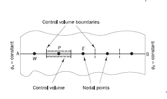
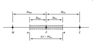
`f_e = { (f_p , if (v.n)_e >0)(f_E , if (v.n)<0)`

If the flow is along -X direction, then the values for this at the interface is given by

for `I_c= v(u_i -u_i-1 )/(Deltax)`which is equivalent to Backward Difference aScheme

If the flow is along +X direction, then the values for this at the interface is given by

for `I_c = v(u_(i+1)-u_i)/(Deltax)`

which is equivalent to Forward Difference Scheme

It is said to be equivalent because all these three methods are of order of accuracy 1.

Advantages:

• UDS is the only approximation that satisfies boundedness criterion unconditionally irrespective of velocity and grid spacing i.e. never yield oscillatory solutions.

Disadvantages:

• UDS is numerically diffusive

Numerical diffusion is magnified in multi-dimensional problems if flow is oblique to the grid.

Peaks or rapid variations in the variables will be smeared out.

• Only first order accurate. Hence very fine grids are required to obtain accurate solutions.

2. Linear interpolation (CDS)

Approximate values of the variable at the control volume face centre by the linear interpolation of the values at the two nearest computational nodes.

`f_e = f_E*lambda_e+F_p(1-lambda)`

and where `lambda_e =(x_e-x_p)/(x_E-x_P)`

`u_(i-1/2)= (u_(i-1)+u_i)/2`

`u_(i+1/2)= (u_i+u_(i+1))/2`

`I_c= v(u_(i+1)-u_(i-1))/(2Deltax`

It is simple and most widely used.

The linear interpolation is equivalent to the use of central difference formula of the firs order derivative and hence this scheme is aslo termed as Central Differencing Scheme(CDS).

which is equivalent to CDS

It is said to be equivalent because both these methods are of order of accuracy 2.

Advantages:

• Approximation of gradients has second order of accuracy on uniform grids
• It's formally of first order on non-uniform grids.

Disadvantages:

• It may produce oscillatory solutio

  Flux limiters:

  When we are calculating Gradients,the values should be bounded they cannot be jumped.If we have a shock flow problem there will be a huge discontinuity, so the gradient will have a huge value ,so will use flux limiter.

  The behaviour of numerical schemes in order to capture shocks and discontinuity that arises in hyperbolic equations. Physically, these equations model the convective fluid flow. It has been observed that low-order schemes are usually stable but quite dissipative in nature around the points of discontinuity/shocks. On the other hand higher-order numerical schemes are unstable in nature and show oscillations in the vicinity of discontinuity. One can have a better understanding of such behaviour by analysing the modified equation of these schemes.

  Now as said above one can not have high order accuracy without oscillations. The objective is to have highly accurate and stable oscillation free schemes. This kind of schemes are known as high resolution schemes. In 1984 Harten proposed the constuction and gave TVD criteria for such scheme. Here we talk only about using flux limiters function to construct high resolution schemes. The idea is to tune the numerical flux of high order and low order scheme using the flux limiter function in such a way that the resulting scheme gives a high order accuracy in the smooth region of flow and sticks with first order of accuracy in the vicinity of socks/discontinuities.

  For convective fluid flow, it is ovservedthat low order schemes are usually stable but quite dissipative in nature around the points of discontinuity or shocks while the higher order schemes are unstable in nature and show oscillations in the vicinity of dinscontinuity or shocks. Highly accurate and oscillation free schemes are known as High Resolution Schemes.

  In order to make the scheme TVD, we must constrain or limit the range of possible values of the additional convective flux

  Average interface values are given by

`f_e = f_p+1/2psi(r)(f_E+f_P)`

`F(u_(i+1/2)) = f^(low)(i+1/2) -psi(r)(f^(low)(i+1/2)-f^(high)(i+1/2))`

`F(u_(i-1/2)) = f^(low)(i-1/2) -psi(r-1)(f^(low)(i+1/2)-f^(high)(i+1/2))`