Project 2 - Rankine cycle Simulator

OBJECTIVE :

• TO Create a Rankine Cycle Simulator MATLAB.
• MY code calculate the state points of the Rankine Cycle (any type of your choice) based on user inputs.

WORKING OF THE RANKINE CYCLE:

**** THE NOTATIONS USED IN THE DIAGRAM AND THE H-S DIAGRAM ARE DIFFERENT FROM EACH OTHER I AM USING DIFFERENT CYCLE METHOD TO CALCULATE THE POINTS.

i.e point 3 shown in h-s diagram is my first point 3=1;

4=2;

1=3;

2=4;

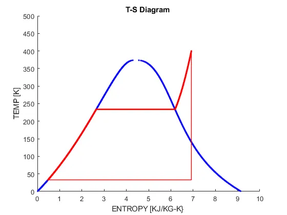
There are four processes in the Rankine cycle. The states are identified by numbers (in brown) in the t-s diagram.

• Process 1–2: The working fluid is pumped from low to high pressure. As the fluid is a liquid at this stage, the pump requires little input energy.

In other words Process, 1-2 is [Isentropic compression]

• Process 2–3: The high-pressure liquid enters a boiler, where it is heated at constant pressure by an external heat source to become a dry saturated vapor. The input energy required can be easily calculated graphically, or numerically, by steam tables.

In other words Process 2-3 is [Constant pressure heat addition in boiler]

• Process 3–4: The dry saturated vapor expands through a turbine, generating power. This decreases the temperature and pressure of the vapour, and some condensation may occur. The output in this process can be easily calculated using the chart or tables noted above.

In other words Process, 3-4 is [Isentropic expansion]

• Process 4–1: The wet vapor then enters condenser, where it is condensed at a constant pressure to become a saturated liquid.

In other words Process 4-1 is [Constant pressure heat rejection in condenser]

In an ideal Rankine cycle, the pump and turbine would by isentropic, i.e., the pump and turbine would generate no entropy and hence maximize the net work output. Processes 1–2 and 3–4 would be represented by vertical lines on the T-S diagram and more closely resemble that of the carnot cycle. The Rankine cycle shown here prevents the state of the working fluid from ending up in the superheated vapor region after the expansion in the turbine, which reduces the energy removed by the condensers.

The actual vapor power cycle differs from the ideal Rankine cycle because of irreversibilities in the inherent components caused by fluid friction and heat loss to the surroundings; fluid friction causes pressure drops in the boiler, the condenser, and the piping between the components, and as a result the steam leaves the boiler at a lower pressure; heat loss reduces the network output, thus heat addition to the steam in the boiler is required to maintain the same level of net work output.

Variables

EQUATIONS:

turbine work

`W_t = H1-H2`

heat input

`Q_in = H1-H4`

work of pump

`W_p = H4-H3`

heat rejected

`Q_out = H2-H3`

thermqal efficiency

`eta_eff = (W_n/Q_i)*100;`

specific steam consumption

`SSC = (3600/W_n)`

back work ratio.

`BW_R = (W_p/W_t);`

where

w_p is the work done by pump

w_t work done by turbine

q_in input by the boiler

q_out heat rejected by condensor

ete_eff thermal efficiency of the plant

SSC specific heat consumption

BWR back work ratio.

X = (S2-SF2)/(SG2-SF2);

x dryness fraction of the steam

s2 entropy at the inlet of condenser outlet of the turbine.

sf2 ENTROPY OF SATURATED FLUID(LIQUID).

sg2 ENTROPY OF SATURATED gas (vapour).

H2 = HF2+ X*(HG2-HF2);

h2 enthalpy of the point 2i.e outlet of the turbine,

hf2 is the enthalpy of the saturated fluid

hg2 enthalpy of the saturated gas

PROGRAMMING LOGIC

• by frintf command, we are showing the state points of the following we are using and writing the program on Rankine cyce.
• 1-2 is the process of isentropic expansion in which the enroy of the system remains constant i.e s1=s2.
• 2-3 is the process of constant pressure heat rejection takes place in the point 2.
• 3-4 is the process of the isentropic compression the compression occurs and the volume changes.
• 4-1 is the process of constant pressure heat addition.
• we are calculating the efficiency of the Rankine cycle, work is done by the turbine, work done by the pump, back work ratio. and specific steam consumption.
• the pressure at the inlet of the turbine is given that is p1= 30;
• the temperature at the inlet of the turbine is given that is p1= 400;
• the pressure at the outlet of the turbine is given that is p2= 0.05;
• we have to download the XStream library function for calculation of the enthalpy, entropy, temperature, volume, at each point has to be calculated in order to plot the T-S and H-S diagram for each state point the everything is to be calculated then only we can get the curve and we can know the efficiency of the Rankine cycle.
• at state point1

H1 = XSteam('h_pt',T1,T1) ENTHALPY AT TURBINE INLET.
S1 = XSteam('s_pt',P1,T1) ENTROPY AT TURBINE INLET.
HF1 = XSteam('hL_p',P1) ENTHALPY OF SATURATED LIQUID.
HG1 = XSteam('hV_p',P1) ENTHALPY OF SATURATED VAPOUR.
TS1 = XSteam('Tsat_p',P1) SATURATED TEMPERATURE.
SF1 = XSteam('sL_p',P1) ENTROPY OF SATURATED FLUID (LIQUID).
SG1 = XSteam('sV_p',P1) ENTROPY OF SATURATED VAPOUR (GAS).

at state point 1 we are calculating these value, the notations are mentioned, from the xsteam table we can calculate the required value as the function of pressure and temperature, or as a function of enthalpy or entropy.

• at state point 2 we have to calculate the value of dryness fraction and by that value, we have to calculate the value of h2 i.e enthalpy at state point 2
• x is the dryness fraction, X = (S2-SF2)/(SG2-SF2)

s2 is the entropy of the fluid at the exit of the turbine.

sf2 is the entropy of the saturated fluid.

sg2 is the entropy of the saturated gas or vapor.

• after calculating these, as usual, we are calculating and moving to the calculation of the some important parameters.
• at state point three we are going to calculate some parameters we are using to drawing the graph of h-s and t-s diagram.
• at state point three the.

H3 = HF2; ENTHALPY AT POINT 3 IS NOTHING BUT ENTTHALPY OF FLUID AT POINT 2
S3 = SF2; ENTROPY IS NOTHING BUT ENTROPY OF FLUID AT POINT 2
T3 = T2; TEMPERATURE AT OUTLET OF TURBINE IS EQUAL TO TEMPERATURE AT INLET ODF CONDENSER BECAUSE WE ASSUME THERE IS NO HEAT LOSS TO THE SURROUNDINGS OF ENVIRONMENT
P3 = P2; P2=P3 BECAUSE IT PRESENT IN THE CONSTANT PRESSURE LINE THE PRESSURE DO NOT CHANGE FROM OUTLET OF TURBINE TO THE INLET OF CONDENSOR

• at state point 4
• as usual, we are calculating the important parameters to make the curve and graph fit in the correct way.

P4 = P1; %p1=p4 because the otlet of boiler is inlet ofdf turbine
S4 = S3; %the entropy is constant at the point
H4 = XSteam('h_ps',P4,S4); % finding the h4 bt xstem library function
T4 = XSteam('T_ps',P4,S4); %t4 finding the temperature at outlet from boiler

we taken p1 = p4 because the pressure at the outlet of the boiler is equal to the pressure at the inlet of the turbine . the steam comes out of the boiler outlet goes to turbine inlet so we consider p1=p4 .

s4=s3 because it the constant entropy line the entropy remains constant in this region i.e there is no pressure loss occurs in the following region

*we are-finding the value of the enthalpy of point 4 by using the xsteam library function.

*and we are calculating the value of temperature at the end boiler output.

• we are going to plot the graph of the liquid saturation curve and vapour saturation curve.
• in which we are plotting the point by taking the teperature value from 400 and we plot against entropy of liquid at sturation point and enropy of gas at saturation point.
• i i=1:length(t)
  plot( XSteam('sL_T',t(i)),t(i),'.','color','b')
  plot( XSteam('sV_T',t(i)),t(i),'.','color','b')
  
  
• we using t(i) because t is varying every time we start plotting it runs about 400 times to the value of the temperature.
• we are plotting for enthalpy and temperature i.e

plot([S2 SG2 S3 S4],[T1 TS2 T3 T4],'linewidth',1,'color','r')

plot([S2 S3 S4],[T2 T3 T4],'linewidth',1,'color','r')

• this plotting made our curve coplete for t-s daaigram

now we have to plot the graph for the h-s daigram i,e entropy vs enthalpy curve

i.e plot(XStream('s_pT',P1,l(i)),l(i),'.','color','r')

this is the plot of the enthalpy and the entropy.

we already calculated all the requirements of the calculation of work done by the turbine, pump, and calculation of network, specific steam consumption, and back work ratio.

then we calculate the heat input, heat rejected by the condenser,

CODE;

% the process going on in the rankine cycle
fprintf('\n  RANKINE CYCLE')
fprintf('\n  1-2 ISENTROPIC EXPANSION')
fprintf('\n  2-3 CONSTANT PRESSURE HEAT REJECTION')
fprintf('\n  3-4 ISENTROPIC COMPRESSION')
fprintf('\n  CONSTANT PRESSURE HEAT ADDITION')

%THE INPUTS ARE GIVEN 

P1 = 30;      %PRESSURE AT INLET OF TURBINE (PRESSURE AT OUTLET OF BOILER).
T1 = 400;     %TEMPERATURE AT INLET OF TURBINE (PRESSURE AT OUTLET OF BOILER). 
P2 = 0.05;    %PRESSURE AT ENTRANCE OF CONDENSOR(OUTLET OF TURBINE).


%At state point 1
%TS1 IS NOTHING BUT INLET TEMPERATURE OF TURBINE

H1  =   XSteam('h_pt',T1,T1) % ENTHALPY AT TURBINE INLET.
S1  =   XSteam('s_pt',P1,T1)   % ENTROPY AT TURBINE INLET.
HF1 =   XSteam('hL_p',P1)      % ENTHALPY OF SATURATED LIQUID.
HG1 =   XSteam('hV_p',P1)      % ENTHALPY OF SATURATED VAPOUR.
TS1 =   XSteam('Tsat_p',P1)    % SATURATED TEMPERATURE.
SF1 =   XSteam('sL_p',P1)      % ENTROPY OF SATURATED FLUID (LIQUID).
SG1 =   XSteam('sV_p',P1)      % ENTROPY OF SATURATED VAPOUR (GAS).

%At state point 2

S2   =  S1;
SF2  =  XSteam('sL_p',P2);     %ENTROPY OF STURATED FLUID(LIQUID).
SG2  =  XSteam('sV_p',P2);     %ENTROPY OF STURATED VAPOUR(GAS).

X    = (S2-SF2)/(SG2-SF2);     % DRYNESS FRACTION

HF2  =  XSteam('hL_p',P2);     %ENTHALPY OF FLUID AT OTLET OF TURBINE OR (INLET OF CONDENSOR).
HG2  =  XSteam('hV_p',P2);     %ENTHALPY OF GAS AT OTLET OF TURBINE OR (INLET OF CONDENSOR).

H2   =  HF2+ X*(HG2-HF2);      %ENTHALPY  OUTLET OF TURBINE OR (INLET OF CONDENSOR).

T2   =  XSteam('T_ph',P2,H2);  %TEMPERATURE AT CONDENSOR INLET OR TURBINE INLET.
TS2  =  XSteam('Tsat_p',P2);   % STURATION TEMPERATURE AT POINT 2.

% At state point 3

H3 =  HF2;                     %ENTHALPY AT POINT 3 IS NOTHING BUT ENTTHALPY OF FLUID AT POINT 2  
S3 =  SF2;                     %ENTROPY IS NOTHING BUT ENTROPY OF FLUID AT POINT 2
T3 =  T2;                      %TEMPERATURE AT 
P3 =  P2;


% At state point 4

P4 = P1;                      %p1=p4 because the otlet of boiler is inlet ofdf turbine
S4 = S3;                       %the entropy is constant at the point 
H4 = XSteam('h_ps',P4,S4);    % finding the h4 bt xstem library function 
T4 = XSteam('T_ps',P4,S4);    %t4 finding the temperature at outlet from boiler




% Calculations

% TURBINE WORK (W_t)

W_t = H1-H2;

% PUMP WORK (W_p)

W_p = H4-H3;


% Heat Addition (Q_in)

Q_in = H1-H4;

% Heat rejection (Q_out)

Q_out = H2-H3;


% Net work done (W_net)
W_net = W_t - W_p;

% Thermal efficiency of the turbine (Therm_eff)

Therm_eff = (W_net/Q_in)*100;

% Specific Steam Consumption (SSC)
SSC = (3600/W_net);

% Back Work Ratio (BW_R)
BW_R = (W_p/W_t);



%FOR CURVE PLOT

t = linspace(0,400,500) % Temp


% T-S DIAGRAM plotting

figure(1)
hold on

% saturation curve
 

for i = 1:length(t)
    STL(i) = XSteam('sL_T',t(i))
    STV(i) = XSteam('sV_T',t(i))
   
end
plot(STL,t,'.','color','b')
   plot(STV,t,'.','color','b')
 
% Cycle plot

plot([S1 S2],[T1 T2],'linewidth',1,'color','r')
if x>1
    T3 = Ts2;
    plot([S2 SG2 S3 S4],[T1 TS2 T3 T4],'linewidth',1,'color','r')
    T2 = TS2;
else
    plot([S2 S3 S4],[T2 T3 T4],'linewidth',1,'color','r')
   
end

l = linspace(T1,T2,1000);

for i = 1:length(l)
    plot(XSteam('s_pT',P1,l(i)),l(i),'.','color','r')
end


plot([SF1 SG1],[TS1 TS1],'linewidth',2,'color','r')
xlabel('ENTROPY [KJ/KG-K} ')
ylabel(' TEMP [K] ')
title('T-S Diagram ')
xlim([0 10]);
ylim([0 500]);


% H-S Diagram Plotting

figure(2)
hold on


figure(2)

for i = 1:length(t)
    plot(XSteam('sL_T',t(i)),XSteam('hL_T',t(i)),'*','color','b')
    plot(XSteam('sV_T',t(i)),XSteam('hV_T',t(i)),'*','color','b')
end

% Cycle plot

plot([S1 S2 S3 S4 S1],[H1 H2 H3 H4 H1],'linewidth',2,'color','r')
xlabel('ENTROPY [KJ/KG-K] ')
ylabel(' ENTHALPY [KJ-KG] ')
title('H-S Diagram')

RESULTS;

the figure

\

this is the t_s diagram of the Rankine cycle. this shows us the variation of the temperature and enthalpy upon the Rankine cycle the two curves shows us the. first curve is the curve of liquid saturation , and the second curve is the saturation curve of the vapour saturation.

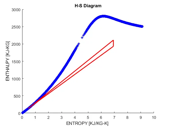
the second plot is the plot of the entropy vs enthalpy we are getting the triangle we connect the 4 point which we got from the calculation of the enthalpy and entropies. i.e

plot([S1 S2 S3 S4 S1],[H1 H2 H3 H4 H1],'linewidth',2,'color','r')
xlabel('ENTROPY [KJ/KG-K] ')
ylabel(' ENTHALPY [KJ-KG] ')
title('H-S Diagram')

by connecting these points we can get the required curve .

CONCLUSION: after attending this session we able to calculate the requirements of t-s and h-s diagram and we know how the ranlkine cycle works.