Week 4 - Genetic Algorithm

OBJECTIVE:

Write a code in MATLAB to optimise the stalagmite function and find the global maxima of the function.

EXPLANATIONS:

• Clearly expalin the concept of genetic algorithm in your own words and also explain the syntax for ga in MATLAB in your report.

INITIALIZATION OF THE POPULATION OR ALSO (CODING):

• Every gene represents a parameter (variables) in the solution. This collection of parameters that forms the solution is the chromosome. The population is a collection of chromosomes.
• Order of genes on the chromosome matters.
• Most of the time chromosomes are depicted in binary as 0’s and 1’s, but there are also other encodings possible.

FITNESS OF FUNCTION:

• Out of the available chromosomes, we have to select the best ones for the reproduction of offsprings, so each chromosome is given a fitness value.
• The fitness score helps to select the individuals which will be used for reproduction.

SELECTION:

• The main goal of this phase is to find the region where the chances of getting the best solution are more.
• Inspiration for this is from the survival of the fittest.
• It should be a balance between exploration and exploitation of search space.
• GA tries to move the genotype to higher fitness in the search space.
• Too strong fitness selection bias can lead to sub-optimal solutions.
• Too little fitness bias selection results in unfocused search.
• Thus Fitness proportionate selection is used, which is also known as roulette wheel selection, is a genetic operator used in genetic algorithms for selecting potentially useful solutions for recombination.

REPRODUCTIO:

reproduction(crossover) is the most vital stage in the genetic algorithm. During reproduction(crossover), a random point is selected while mating a pair of parents to generate offsprings.

There are 3 major types of crossover.

• Single Point Crossover: A point on both parents’ chromosomes is picked randomly, and designated a ‘crossover point’. Bits to the right of that point are exchanged between the two parent chromosomes.
• Two-Point Crossover: Two crossover points are picked randomly from the parent chromosomes. The bits in between the two points are swapped between the parent organisms.
• Uniform Crossover: In a uniform crossover, typically, each bit is chosen from either parent with equal probability.

The new offspring are added to the population.

STOPPING CRITERIA: this must be refers to the condition that must be reach to stop the execution of algorithm.

some of the stopping conditions are

execution time, number of iteration , non improving iterations,

optimal (lower bound for min, upper bound for max) solution found, etc.

SYNTAX OF GA:

x=ga(fun,nvars)

x=ga(fun,nvars,a,b)

EQUATIONS:

`f1,x=(sin(5*pix+0.5))^6`

`f1,y=(sin(5*piy+0.5))^6`

`f2,x=exp(-4*log(2)*(x-0.0667)^2/(0.64))`

`f2,y=exp(-4*log(2)*(x-0.0667)^2/(0.64))`

`f =(f1,x*f1,y*f2,x*f2,y)`

CODE:

code1:

% DE3FINING SEARCH SPACE

clear all; close all; clc

x=linspace(0,0.6,150);
y=linspace(0,0.6,150);          %for x,y we are giving the values of 0- 0.6 and the values beween 0-0.6 are divided into 150 parts thsts what the linspace comment do. 

%defining 2d array

[xx yy]=meshgrid(x,y);     %meshgrid comment is used to create 2d dimentional array of y and y values , the marrix contains x rows and y values

%evaluating stalagmite function

for i=1:length(xx);
    
    for j=1:length(yy);
        
        input_vector(1)=xx(i,j);    % for loop is used to repeat the same operations for multiple options 
        
        input_vector(2)=yy(i,j);    % input vectors 1,2 storing the value of x and y in the in it
        
        f(i,j)=stalagmite_func(input_vector);
        
    end
    
end

xlabel('xvalue')
ylabel('yvalue')
surfc(xx,yy,f)            % surfc command is used to plot the 3d graph for the given data

shading interp            % shading interp
[inputs, fval] =  ga(@stalagmite_func,2)

function for code1:

We are creating the function in the name of stalagmite_function the value of input vector is taken from the stalagmite_func

We are assining the value to x.

We are assining the value of y.

We are explaining the the value of f1_x by the formula.

We are explaining the the value of f1_y by the formula .

Then we are assining the value to f2_x by the formula we is given.

Then we are assining the value to f2_y by the formula we is given.

Then we are using all.parameters to give the value for stalagmite i.e -(f1_x.*f2_y.*f3_x.*f4_y).

Then we end the function.

function [stalagmite]= stalagmite_func(input_vector)

x=input_vector(1);

y=input_vector(2);


f1_x=sin(5*pi*x+0.5)^6;

f2_y=sin(5*pi*y+0.5)^6;

f3_x=exp((-4*log(2)).*(x-0.0667).^2./0.64);

f4_y=exp((-4*log(2)).*(y-0.0667).^2./0.64);


stalagmite =-(f1_x.*f2_y.*f3_x.*f4_y);

end

code2.

*Asusual we are creating the program by clearing and closing all the data which is stored in work space.

We are assining the value to x and y using the linspace command between 0 to 0.6 and value will be divided into 150 parts.

We are running 50 cases here. So

We taking the value of x,y from the stalagmite get_stalagmite.

We are running the for loop for unbounded conditions.

We are using the tic toc command to calculate the time when the code is running.

clear all
close all
clc

x=linspace(0,0.6,150);   %linspace command ised to divide value x and y in between
y=linspace(0,0.6,150);
num_cases=50;
f=get_stalagmite(x,y);


      

tic 
%STUDING THE STATISTICAL BEHAVIOUR OF THE MINIMUM FUNCTION

 for i=1:num_cases
     [inputs,fopt(i)]=ga(@stalagmite_func,2);
     xopt(i)=inputs(1);                         %we are running the stalgmite function here using the for lop . the loop is uased to run the code many times
     yopt(i)=inputs(2);
     
 end
    
     study_time= toc
     
     figure(1)
     subplot(2,1,1)            %figure command is used to made first figure.
     hold on                   %hold on is used to over lap the curve 
     surfc(x,y,-f)              %surfc  is used to plot th 3d plot
     shading interp            %shading interp is used to takeing off the grid lines
     plot3(xopt,yopt,-fopt,'marker','o','markersize',5,'markerfacecolor','r') %plot command is used to plot the graph 
     xlabel('x')
     ylabel('y')              %label command is used to label rthe axis
     
     title('unbounded inputs') % title command is uded to name the plot. 
     subplot(2,1,2)             %subplot command is used to make3 plot wintin the 1 graph.
     plot(-fopt)
     xlabel('iterations')        %label is used to label the axis
     ylabel('function minimum')
     
     
        
     
     tic
     %STUDY_ 2 WITH UNDER AND LOWER BOUND VALUES BY ADDING CONSTRAINTS
     
     
     for i =1:num_cases
         [inputs,fopt(i)]=ga(@stalagmite_func,2,[],[],[],[],[0;0],[0.6;0.6]);
         xopt(i)=inputs(1);
         yopt(i)=inputs(2);
         
     end
         
     study_time=toc                 
     
     figure(2)                   %figure command is used to made first figure.           
     subplot(2,1,1)                 %hold on is used to over lap the curve 
     hold on
     surfc(x,y,-f)                   %surfc  is used to plot th 3d plot
     shading interp                  %shading interp is used to takeing off the grid lines
     plot3(xopt,yopt,-fopt,'marker','o','markersize',5,'markerfacecolor','r')
     xlabel('x')                     %label command is used to label rthe axis
     ylabel('y')
     subplot(2,1,2)                 %subplot command is used to make3 plot wintin the 1 graph.
     xlabel('iteration')             %label command is used to label rthe axis
     ylabel('function minimum')
     plot(-fopt)
     
     %STUDY 3 INCREASING GA ITERATIONS AND CONSTRAINTS
     
     options=optimoptions('ga')
     options=optimoptions(options,'populationsize',300);
     
     
     tic
     
     for i=1:num_cases
         [inputs,fopt(i)]=ga(@stalagmite_func,2,[],[],[],[],[0;0],[0.6;0.6],[],[],options);
         xopt(i)=inputs(1);
         yopt(i)=inputs(2);
     end
     
     study_time=toc
     
     
     figure(3)           %figure command is used to made first figure.
     subplot(2,1,1)
     plot3(xopt,yopt,-fopt,'marker','o','markersize',5,'markerfacecolor','r')
     xlabel('x')          %label command is used to label rthe axis
     ylabel('y')
     hold on             %hold on is used to over lap the curve 
     surfc(x,y,-f)         %surfc  is used to plot th 3d plot
     shading interp       %shading interp is used to takeing off the grid lines
     subplot(2,1,2)       %subplot command is used to make3 plot wintin the 1 graph.
     xlabel('iterations')
     ylabel('function minimum')   %label command is used to label rthe axis
     plot(-fopt)
     

function code 2:

function [q]= get_stalagmite(x,y)

[xx yy]=meshgrid(x,y)


 f1_x=(sin(5*pi.*xx+0.5)).^6

 f1_y=(sin(5*pi.*yy+0.5)).^6

 f2_x=exp((-4*log(2)).*(xx-0.0667).^2./0.64);

 f2_y=exp((-4*log(2)).*(yy-0.0667).^2./0.64);


[q] =-(f1_x.*f1_y.*f2_x.*f2_y);
end

RESULTS;

figure(1): this graph showing the local minima local maxima , global minima,maxima values by using the stalagmite function we can predict x and y values at any point we where the local,global minima,maxima is occuring.

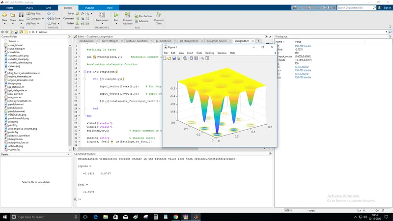
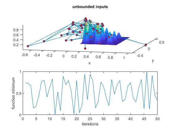
uncomprees condition

with less number of irerations the results are taken fron the programme. the poulation are founding ooutside of domain also so we have to mae the within the domain.

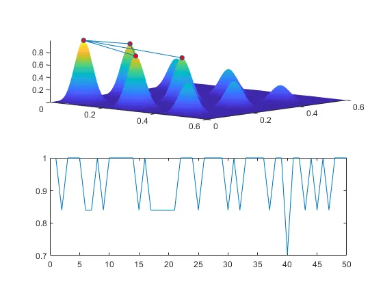
now in this figure we are getting the constraints within the domain but we have to calculate the constraints within the domain

now in this figure we are calucating the local maxima of the point we ate doing more number of iterations and also giving the population size to the constraints as the poulation size increases the computing time also increases and we can find the constraints exactly.

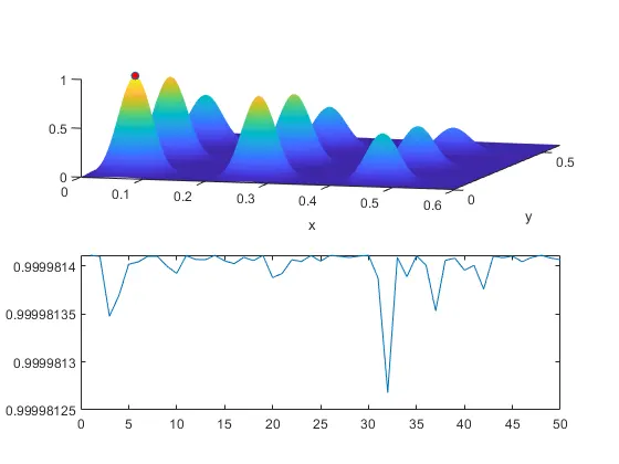
CONCLUSION; after doing this programme we are able to calculate the constraints with in the given domain the value of loacal maxima and minima, and the value of global maxima and minima are also calculated through this method