Week 7 - Simulation of a 1D Super-sonic nozzle flow simulation using Macormack Method
Flow-Through Nozzle
Introduction to Nozzle
A nozzle is a device designed to control the direction or characteristics of a fluid flow (to increase velocity) as it exits (or enters) an enclosed chamber or pipe. A nozzle is often a pipe or tube of varying cross-sectional area, and it can be used to direct or modify the flow of a fluid(liquid or gas). Nozzles are frequently used to control the rate of flow, speed, direction, mass, shape, and pressure of the stream that emerges from them. In a nozzle, the velocity of the fluid increases at the expense of its pressure energy.
Flow-through nozzles occurs in a variety of engineering applications:
- Convergent nozzles are used for subsonic and sonic flows. They can also be used as flow measuring and flow regulating devices.
- Convergent-Divergent nozzles are used for Supersonic flows. It is comparatively difficult to obtain convergent-divergent passages in compressors and turbine blade rows.
Here we are interested in the Convergent-Divergent nozzle as we are writing a code to solve the 1D Supersonic nozzle flow equations using Macormack Method.
Abstract : Set up of a time marching, finite difference solution for the Quasi 1D subsonic supersonic nozzle flow. Non-dimensionalizing the Governing flow equations and setting them up with relevant initial and boundary conditions and solving using the Maccormacks technique. Simulating the solution for convergence and comparing the normalized mass flow rate between Non-conservative and Conservative forms and making conclusions. Performing grid dependence test.
I. Introduction :
We consider the steady state, isentropic flow through convergent-divergent nozzle as shown below. The flow at inlet to the nozzle comes from a reservoir. The cross-sectional area of the reservoir is large and hence the velocity is very small. Thus pressure and temperature at reservoir are stagnation values or total pressure and total temperatures, respectively. The flow expands isentropically to super-sonic speeds at nozzle exit. The flow is locally subsonic in the convergent section of the nozzle and sonic at the throat and supersonic at the divergent section. The sonic flow is M=1 , where M is mach no. means that local velocity at this location is equal to local speed of sound.
The area of nozzle changes as a function of distance along the nozzle (x), we make the assumption that the flow properties vary only with x, to assume uniform flow properties accross any given cross section. Such flow is defined as quasi-one-Dimensional.
II. Project Objectives :
- Write matlab code to Simulate and solve 1D subsonic supersonic nozzle flow equations using MacCormacks method.
- Implementing both Conservative and Non conservative forms of governing equations and making seperate functions both forms.
- To find out minimum number of cycles for which the simulation should be run to achieve convergence.
- Compare the normalized mass flow rate between Conservative and Non-conservative forms
- Timewise variations of density, temperature, velocity and mach no at nozzle throat.
- Distribution of Mass flow through nozzle at different times during time-marching approach to steady state.
- Perform grid dependence test.
III. Governing Flow equations (Non-Dimensional variables) :
Defining the Non-Dimensional variables as,
Temperature : `T' = T_0/T`
Density : `rho' = rho/rho_0`
Dimensionless length : `x' = x/L`
Speed of sound : `a_0 = sqrt(lambda*R*T_0)`
Velocity:`V' = V/a_0`
Time : `t = t /(t/a_0)`
Area : `a = a/(a_(throat))`
Introducing these Dimensionless variables in the governing flow equations, we get :
III. A) For Non-conservative form :
Continuity equation : `(delrho)/(delt)= -rho((delv')/(delx')) - rho'*v' ((del(lna'))/(delx')) - v ((delrho)/(delx))`
Momentum equation : `(delv)/(delt)= -v ((delv)/(delx))-(1/gamma) ((delt')/(delx')+((T)/(rho'))*(delrho')/(delx'))`
Energy equation : `(delT)/(delt) = -v (delT)/(delx)- (gamma-1)*T [(delv)/(delx)+v'(del(lnA))/(delx')]`
III. B) For Conservative form :
Continuity equation : `(delrho)/(delt)=(del(rho'A'))/(delT') +(del(rho'A'V'))/(delx') =0`
Momentum equation : `(delv)/(delt) = ((del(rho'A'V'))/(delt'))+((del[rho'A'*V^2+(1/gamma)(rho'A'))]/(delx'))=(1/rho) *p'(delA')/(delx')`
Energy equation : `(del[ rho'((e)/(gamma-1)+(lambda/2)*v^2)*aA'])/(delt')+((del[rho'(e)/(gamma-1)+(lambda/2)*v^2)*V'A'+rho' a' v'])/(delx')= 0`
Now, the generic form of equation can be expressed as :
Solution vector : U
Flux term : F
Source term : J
Defining the elements of Solution vector U
`u1= rho'a`
`u2 =rho'a'v`
`u3 =rho ((e)/(gamma-1)+(gamma/2)*v^2)`
PURE FORM OF FLUSX TERMS
`F1 =rho'A' =U1`
`F2=rho'A'v'^2+(1/gamma)p'A'=(U_2)^2/(U_1)+(gamma-1)/(gamma)((U_3)-gamma/2(u_2^2)/u_1)`
`F3=rho'(T/(gamma-1)+(gamma/2)*v'^2)*V'A'=(gammaU_2U_3)/(U_1)+ (gamma(gamma-1))/ 2*(U_2^3)/U_1^3`
`J2 = (gamma-1)/(gamma)(u_3-(gamma/2)(u_2^2)/(u_1))*((del(ln(A)))/(delx')`
after substituting therse terms in governing equation we get
`(delU_1)/(delt')= (-delF_1)/(delx')`
`(delU_2)/(delt')=-(delF_2)/(delx')+J2`
`(delU_3)/(delt') = - (delF_3)/(delx')`
- ABOVE VALUE OF F1,F2,F3 AND J2 ARE PUT IN EQUATION 10,11,12.
CASE SETUP FOR NON-CONSERVATIVE FORM :
- WE GOT GOVERNING EQUATION SHOWN ABOVE (4-n & 5-n & 6-n) WE WILL APPLY MACORMACK TECHNIQUES ON THOSE EQUATION .
- CALCULATION OF TIME STEP :
- `DeltaT= C*(Deltax)/(a+v)` equation is used for calculating time at every node point out minimum value is choosed for DeltaT
- where C= courant no. , a= speed of sound in medium & v= speed of propogating flow
- `DeltaT = min(T^t(1) + T^t(2) +(T^t(3).....)
3. BOUNDARY CONDITION :
1)Inlet boundary :
- v(1)=2⋅v(2)-v(3)">v(1)=2⋅v(2)−v(3)v(1)=2⋅v(2)-v(3) using linear extrapolation at point 1 & 2 & 3
2) Outlet boundary :
- v(n)=2⋅v(n-1)-v(n-2)">v(n)=2⋅v(n−1)−v(n−2)v(n)=2⋅v(n-1)-v(n-2))
- ρ(n)=2⋅ρ(n-1)-ρ(n-2)">ρ(n)=2⋅ρ(n−1)−ρ(n−2)ρ(n)=2⋅ρ(n-1)-ρ(n-2))
- T(n)=2⋅T(n-1)-T(n-2)">T(n)=2⋅T(n−1)−T(n−2)T(n)=2⋅T(n-1)-T(n-2))
4. INITIAL CONDITION :
-
A=1+2.2*(x.">.xx.-1.5).^(2)
-
rho=1-0.3146*x.">.xx.
-
T = 1-0.231*x.">.xx.
-
v=(0.1+1.09*x.">.xx.).*T.^(1/2)
CASE SETUP FOR CONSERVATIVE FORM :
- WE GOT GOVERNING EQUATION SHOWN ABOVE (10 ,11,12) WE WILL APPLY MACORMACK TECHNIQUES ON THOSE EQUATION .
- CALCULATION OF TIME STEP :
- `DeltaT= C*(Deltax)/(a+v)` equation is used for calculating time at every node point out minimum value is choosed for DeltaT
- where C= courant no. , a= speed of sound in medium & v= speed of propogating flow
- `DeltaT = min(T^t(1) + T^t(2) +(T^t(3).....)
3. BOUNDARY CONDITION :
Inlet
U1(1) = rho(1)*a(1)
U2(1) = 2*U2(2)-U2(3)
U3(1) = U1(1)*((T(1)/(gamma-1))+(0.5*gamma*(v(1).^2)))
Outlet
U1(n) = 2*U1(n-1)-U1(n-2);
U2(n) = 2*U2(n-1)-U2(n-2);
U3(n) = 2*U3(n-1)-U3(n-2);
4. INITIAL CONDITION :
- A=1+2.2*(x.">.xx.-1.5).^(2)
for (0<x.">.xx.< 0.5)
ρ.">.ρρ.=1
T.">.TT.=1
for(0.5 <=x.">.xx.<= 1.5)
ρ.">.ρρ.=1-(0.366*(x-0.5))
T.">.TT. = 1-0.167*(x-0.5)
for(1.5 <=x.">.xx.<= 3.5)
ρ.">.ρρ.=0.634-(0.3879*(x-1.5))
T.">.TT.= 0.833-(0.3507*(x-1.5))
3). v.=0.59ρ.⋅A.">.v=0.59.ρ⋅.A
v.=0.59ρ.⋅A.">code:
v.=0.59ρ.⋅A.">main code
main code
clear all
close all
clc
n= 31;
x= linspace(0,3,n);


    a= 1+2.2*(x-1.5).^2  ;  %area vector


    mass_flow_rate_1= non_conservative(a);
    mass_flow_rate_2= conservative(a);


 figure(7)
 plot(x,mass_flow_rate_1)
 hold on
 plot(x,mass_flow_rate_2)
 plot(x,0.58*ones(n,1),'--')
 axis([0 3 0.575 0.6])
 xlabel('non dimentional length')
 ylabel('mass flow rate')
 legend('non conservative form solution','conservative form solution','EXACT SOLUTION')
 title('variation of the mass flow rate along ther length of domain')
non conservative functional code
function [mass_fl_rate] = non_conservative(a)

    %initial conditions
   n= 31;
   x = linspace(0,3,n);
   dx = x(2) - x(1);
    %calculating initial profiles
    rho = 1- 0.3146*x; % density
    t = 1- 0.2314*x;    %temperaturte
    v = (0.1+1.09*x).*t.^0.5 ; %velocity
    a= 1+2.2*(x-1.5).^2  ;  %area vector
    nt = 1400;
    gamma = 1.4;
    c = 0.5;
    %finding the throat area and
    throat = find (a ==1);
        for  k = 1:nt
             dt = min(c*(dx./(sqrt(t)+v)));

            rho_old = rho;
            v_old = v;
            t_old = t;


               %predictor method
            for j = 2:n-1

                dv_dx = (v(j+1) - v(j))/dx;
                dloga_dx = (log(a(j+1))- log(a(j)))/dx;
                drho_dx =  (rho(j+1) - rho(j))/dx;
                dt_dx =  (t(j+1) - t(j)) / dx;

                %continuity equation
                drho_dt_p(j) = -rho(j) *(dv_dx)   - rho(j)*v(j) * (dloga_dx) - v(j)*(drho_dx );

                %$momentum eqaution
                dv_dt_p(j) =  - v(j) *(dv_dx) -  (1/gamma) *  ((dt_dx) + (t(j)/rho(j))*drho_dx);

                %energy equation
                dt_dt_p(j) = - v(j) * (dt_dx)  - (gamma-1)*t(j) * (dv_dx  +  v(j)*dloga_dx);


                 rho(j) = rho(j) + drho_dt_p(j)*dt;

                v(j) = v(j) + dv_dt_p(j) *dt;

                t(j) = t(j) + dt_dt_p(j) *dt;

            end


                %corrector method
                for j = 2:n-1

                dv_dx = (v(j) - v(j-1))/dx;
                dloga_dx = (log(a(j))- log(a(j-1)))/dx;
                drho_dx =  (rho(j) - rho(j-1))/dx;
                dt_dx =  (t(j) - t(j-1)) / dx;

                %continuity equation
                drho_dt_c(j) = -rho(j) *(dv_dx)   - rho(j)*v(j) * (dloga_dx) - v(j)*(drho_dx );

                %$momentum eqaution
                dv_dt_c(j) =  - v(j) *(dv_dx) -  (1/gamma) *  ((dt_dx) + (t(j)/rho(j))*drho_dx);

                %energy equation
                dt_dt_c(j) = - v(j) * (dt_dx)  - (gamma-1)*t(j) * (dv_dx  +  v(j)*dloga_dx);


                 end

            %compute the average time derivative
             drho_dt = 0.5*(drho_dt_p + drho_dt_c);

             dv_dt    = 0.5*(dv_dt_p + dv_dt_c);

             dt_dt    =0.5* (dt_dt_p  +dt_dt_c);


             %solution update
               for j= 2:n-1
                rho(j) = rho_old(j) + drho_dt(j)*dt;

                v(j) = v_old(j) + dv_dt(j) *dt;

                t(j) = t_old(j) + dt_dt(j) *dt;
               end

               % apply boundary condition
               %inlet boundary condition
                v(1) = 2*v(2) - v(3);


               %outlet boundary conduition
               v(n) = 2*v(n-1) - v(n-2);
               rho(n)  = 2*rho(n-1) -rho(n-2);
               t(n) =  2*t(n-1) - t(n-2);


               M = v./sqrt(t);       %match number
               p = rho.*t;           %
               mass_fl_rate = rho.* v.*a;%mass flow rate

               m_throat(k) = M(throat);     %for each time step setting match number is equal to 1 at throat
               p_throat(k) = p(throat);
               mass_throat(k) = mass_fl_rate(throat);
               rho_throat(k) = rho(throat);


              figure(4)

            if k == 50
                plot(x,mass_fl_rate)

                hold on
            elseif k == 100
                plot(x,mass_fl_rate)
                hold on
            elseif k == 150
               plot(x,mass_fl_rate)
                hold on
             elseif k == 200
                plot(x,mass_fl_rate)
                hold on
             elseif k == 400
                plot(x,mass_fl_rate)
                hold on
             elseif k == 700
                plot(x,mass_fl_rate)
                legend('dt = 50','dt = 100','dt = 150','dt = 200','dt= 400','dt = 700')
                xlabel(' NON DIMENTIONAL DISTANCE THROUGH NOZZLEX')
                ylabel('NO DIMENTIONAL MASS FLOW RATE')
                title(sprintf('VARIATION OF MASS FLOW RA    TE WITH THE VARIATION OF THE LENGTH \n (NON CONSERVATIVE FORM)'))
            end
        end


    figure(5)
    subplot(4,1,1)
    plot(m_throat,'b')
    xlabel('no of iterations')
    ylabel('temperatutre')
    title(sprintf('VARIATION OF THE THROAT PROPERTIES vs NUMBER OF ITERATIONS \n(NON CONSEVATIVE FORM)'))
    subplot(4,1,2)
    plot(p_throat,'g')
     xlabel('no of iterations')
    ylabel('density')
    subplot(4,1,3)
    plot(mass_throat','r')
     xlabel('no of iterations')
    ylabel('mach number')
    subplot(4,1,4)
    plot(rho_throat,'cyan')
     xlabel('no of iterations')
    ylabel('pressure')


     figure(6)
    subplot(4,1,1)
    plot(x,M)
    xlabel('NON DIMENTIONAL LENGTH')
    ylabel('mach number')
      title(sprintf('VARIATION PARAMETERS ALONG THE LENGTH OF THE NOZZLE \n (NON CONSERVATIVE FORM)'))

    subplot(4,1,2)
    plot(x,t)
    xlabel('NON DIMENTIONAL LENGTH')
    ylabel('temperature')


    subplot(4,1,3)
    plot(x,rho)
    xlabel('NON DIMENTIONAL LENGTH')
    ylabel('density')

    subplot(4,1,4)
    plot(x,p)
    xlabel('NON DIMENTIONAL LENGTH')
    ylabel('pressure')


 end
conservative functional code
 function [mass_fl_rate] = conservative(a);


    %non conservative form of eqyation

    n = 31;              %number of nodes
    x = linspace (0,3,n); %creating the doomain in parti cular amount of nodes
    dx = x(2) - x(1);

    for i=1:n
        if  (0<=x(i)) && (x(i)<=0.5)

        rho(i)=1;
        t(i)=1;

        elseif (0.5<=x(i)) && (x(i)<=1.5)

        rho(i)=1-(0.366*(x(i)-0.5));
        t(i) = 1-0.167*(x(i)-0.5);

        else

        rho(i) =0.634-(0.3879*(x(i)-1.5));
        t(i) = 0.833-(0.3507*(x(i)-1.5));
        end
    end

    %inputs for calculation of u1,u2, u3
    a= 1+2.2*(x-1.5).^2  ;%area vector


    gamma = 1.4;
    u1 = rho.*a;
    v = 0.59./(u1);
    u2 = (rho.*a).*v;
    nt = 1400;
    u3=(rho.*a).*((t/(gamma-1)+ (0.5*gamma*v.^2)));
    throat = find(a==1);
   c = 0.5;

    for k =1 :nt

        dt = min(c*(dx./(sqrt(t)+v)));

        u1_old = u1;
        u2_old = u2;
        u3_old = u3;

        %flux variables
        f1 = u2;
        f2 = ((u2.^2)./u1) +  ((gamma-1)/gamma) * ( u3 - ((0.5*gamma)*((u2.^2)./u1)));
        f3 = (gamma * ((u3.*u2)./u1))  -  (  (gamma*(gamma-1)/2)*((u2.^3)./u1.^2)  );

            %PREDICTOR  STEP
            for  i = 2 :n-1

                da = (a(i+1) -a(i))/dx;
                j2(i) =(rho(i)*t(i)*da)/gamma;

                du1_dt_p(i) = -(f1(i+1) - f1(i))/dx;
                du2_dt_p(i) = - (f2(i+1) - f2(i))/dx +j2(i);
                du3_dt_p(i) = - (f3(i+1)-f3(i))/dx;


                u1(i) = u1(i) +   du1_dt_p(i)*dt;
                u2(i) = u2(i) +   du2_dt_p(i)*dt;
                u3(i) = u3(i) +   du3_dt_p(i)*dt;

                rho(i) = u1(i)./a(i);
                v(i) = u2(i)./u1(i);
                t(i)  = (gamma-1) *   (   (u3(i)/u1(i)) - (gamma/2)*((u2(i)/u1(i))^2)  );
            end

         f1 = u2;
         f2 = ((u2.^2)./u1) +  ((gamma-1)/gamma) * ( u3 - ((0.5*gamma)*((u2.^2)./u1))) ;
         f3 = (gamma * ((u3.*u2)./u1))  -  (  (gamma*(gamma-1)/2)*((u2.^3)./u1.^2)  );

            %CORRECTOR STEP
         for  i = 2 :n-1

                da = (a(i) -a(i-1))/dx;
                j2(i) =(rho(i).*t(i).*da)/gamma;


                du1_dt_c(i) = -(f1(i) - f1(i-1))/dx;
                du2_dt_c(i) = - (f2(i) - f2(i-1))/dx +j2(i);
                du3_dt_c(i) = - (f3(i)-f3(i-1))/dx;


                u1(i) = u1(i) +   du1_dt_c(i)*dt;
                u2(i) = u2(i) +   du2_dt_c(i)*dt;
                u3(i) = u3(i) +   du3_dt_c(i)*dt;

                rho(i) = u1(i)./a(i);
                v(i) = u2(i)./u1(i);
                t(i)  = (gamma-1) *   (   (u3(i)/u1(i)) - (gamma/2)*((u2(i)/u1(i))^2)  );
         end

         %updating flux values
          du1_dt = 0.5*(du1_dt_p+ du1_dt_c);
          du2_dt = 0.5*(du2_dt_p+ du2_dt_c);
          du3_dt = 0.5*(du3_dt_p+ du3_dt_c);

          for i =2:n-1
               u1(i)= u1_old(i) + du1_dt(i)*dt;
               u2(i)= u2_old(i) + du2_dt(i)*dt;
               u3(i)= u3_old(i) + du3_dt(i)*dt;
          end

               %updating the values of rho, v , t
                rho = u1./a;
                v = u2./u1;
                t  = (gamma-1) *   (   (u3./u1) - (gamma/2)*((u2./u1).^2)  );


                %boundary condition
                %inlet boundary
                u1(1) = rho(1).*a(1);
                u2(1) = 2*u2(2)- u2(3);
                u3(1) = u1(1)*((t(1)/(gamma-1))+(0.5*gamma*(v(1).^2)));

                %outlet boundary
                u1(n) = 2*u1(n-1) - u1(n-2);
               u2(n) = 2*u2(n-1) - u2(n-2);
               u3(n) = 2*u3(n-1) - u3(n-2);

               M = v./sqrt(t);
               p = rho./t;
               mass_fl_rate = rho.*a.*v;

               m_throat(k) = M(throat);
               t_throat(k) = t(throat);
               rho_throat(k) = rho(throat);
               v_throat(k) = v(throat);
               a_throat(k)  = a(throat);

               mass_throat = rho_throat.*a_throat.*v_throat;
               p_throat = rho_throat.*t_throat;

        figure(1)

        grid on
        hold on
        if k==0
            plot(x,mass_fl_rate)

            hold on
        elseif k==100

            plot(x,mass_fl_rate)

            hold on
        elseif k==200

            plot(x,mass_fl_rate)

            hold on
        elseif k ==700

        plot(x,mass_fl_rate)

        hold on
        elseif k ==1000

        plot(x,mass_fl_rate)

        end

        legend('dt = 0','dt = 100','dt= 200','dt = 700')
        title(sprintf('VARITAION OF THE MASS FLOW RATE WITH CHANGE IN TIME STEP '))
        xlabel('LENGTH OF THE NOZZLE')
        ylabel('MASS FLOW RATE')

    end
        figure(2)
    subplot(4,1,1)
    plot(t_throat,'b')
    xlabel('no of iterations')
    ylabel('temperatutre')
    title(sprintf('VARIATION OF THE THROAT PROPERTIES vs NUMBER OF ITERATIONS \n(CONSEVATIVE FORM)'))
    subplot(4,1,2)
    plot(rho_throat,'g')
     xlabel('no of iterations')
    ylabel('density')
    subplot(4,1,3)
    plot(m_throat','r')
     xlabel('no of iterations')
    ylabel('mach number')
    subplot(4,1,4)
    plot(p_throat,'cyan')
     xlabel('no of iterations')
    ylabel('pressure')

    figure(3)
    subplot(4,1,1)
    plot(x,M)
    xlabel('NON DIMENTIONAL LENGTH')
    ylabel('mach number')

    title(sprintf('VARIATION OF PARAMETERS ALONG THE LENGTH OF THE NOZZLE \n (CONSERVATIVE FORM)'))

    subplot(4,1,2)
    plot(x,t)
    xlabel('NON DIMENTIONAL LENGTH')
    ylabel('temperature')


    subplot(4,1,3)
    plot(x,rho)
    xlabel('NON DIMENTIONAL LENGTH')
    ylabel('density')

    subplot(4,1,4)
    plot(x,p)
    xlabel('NON DIMENTIONAL LENGTH')
    ylabel('pressure')


 end
non conservative function code
RESULTS;
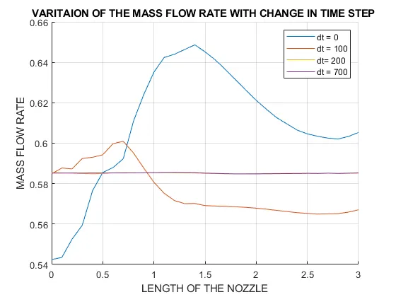
as the time step increases we can get through the convergence. what we mean by this means as the time step increases we can get closer to the exact value and as the timer step incereases, the mas flow arte also goews to reach the steady state. and this graph also shows that we can go to converge after 600 iterations
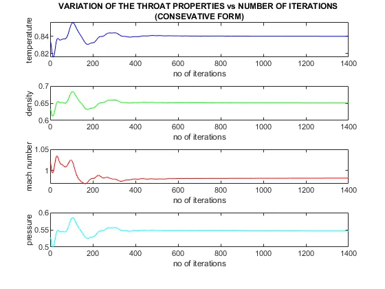
this is the comparison of the of the mach number and, density, pressure temperature,
we know that *as the iteration are getting increased as the we reach the steady state means there is no change in the properties of the after the flow inside the nozzle reach the stedy state . means the flow properties at each points are same as compared to other point. it is only happen after some time i.e after the number of time step is more than 700. or we can increase rthe number of the grid points
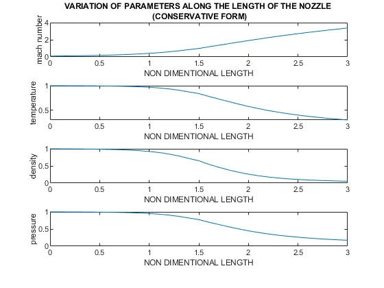
as the are is convergent the are going to become smaller after each time step . and we know the if area become smaller the pressure will increase and as the pressure ijncreases the the tempereture is also going to increase . and density also
but at the outlet area becomes increasing and as aa result the density decreases and the temperature decreases a density also decreases and but mech number increases.
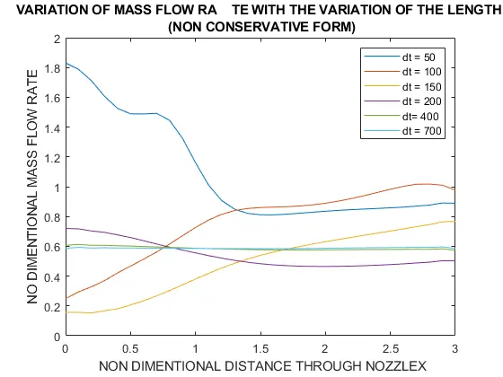
as the time step increases we can get through the convergence. what we mean by this means as the time step increases we can get closer to the exact value and as the timer step incereases, the mas flow arte also goews to reach the steady state. and this graph also shows that we can go to converge after 600 iterations
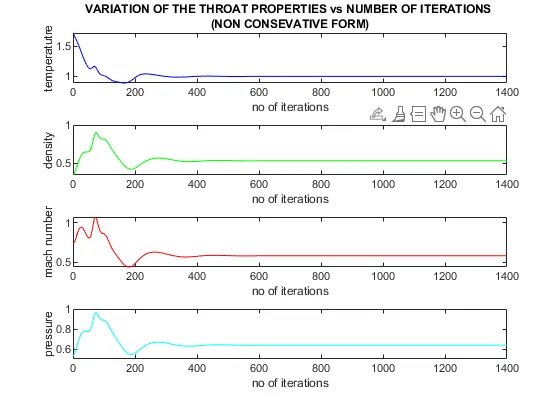
this is the comparison of the of the mach number and, density, pressure temperature,
we know that *as the iteration are getting increased as the we reach the steady state means there is no change in the properties of the after the flow inside the nozzle reach the stedy state . means the flow properties at each points are same as compared to other point. it is only happen after some time i.e after the number of time step is more than 700. or we can increase rthe number of the grid points
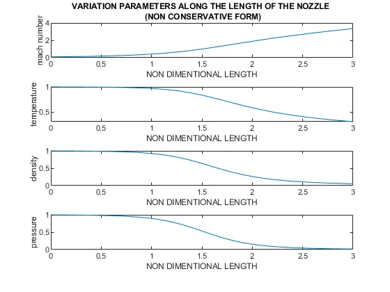
as the are is convergent the are going to become smaller after each time step . and we know the if area become smaller the pressure will increase and as the pressure ijncreases the the tempereture is also going to increase . and density also
but at the outlet area becomes increasing and as aa result the density decreases and the temperature decreases a density also decreases and but mech number increases.
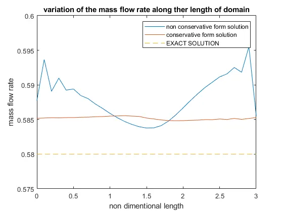
this graph showing the comparision of the solutions of the both conservative and the non conservative form , the difference between the conservative and non conservative form is very little as shown in the graph or curve bopth are nearly equal to exact solution
FOR GRID INDEPENDENCE TEST WE INCREASE THE VALUE OF THE NUMBER OF GRID POINTS THEN WE CAN GET THE GET RESULTS ARE SUTAIBLE
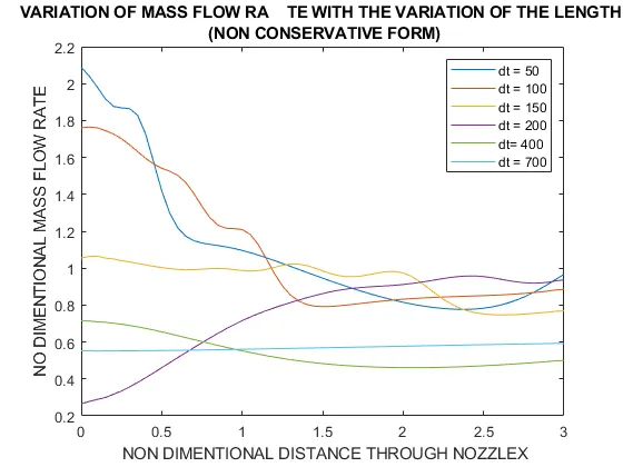
for the mass flow rate the curves become more smoother and more lineat if we increase the number of grid points by 30 we can further increase the grid points. if we incraase the grid points further the solution become more stable and pointed near to exact solution.
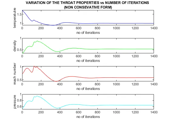
this are the variation of the throat properties with increase in the number of the grid points the solution is more smoother than previous results and . as the number of grid points increases the accuracy of the solution also increases. the oscillation become lesser
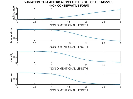
the mach number temperature, density,pressure, are the properties of the fluid which is flowing through the nozzle. as the length of the nozzle changes. during the convergent stage the fluid properties increase like temperature increases as the pressure increases, the and during the divergent stage the pressure decreases as the area increases and as the pressure decreases the temperature also decreases and the density also decreases as the area increases.
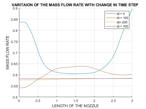
this is the curve of them,ass flow rate as the we increase the number of the grid points the mass flow rate is going to attain steady state.as the we increase the number of the3 grid points . we get convergence rate is lesser than that of the when we use the lesser numbwer of tyhe grid points.
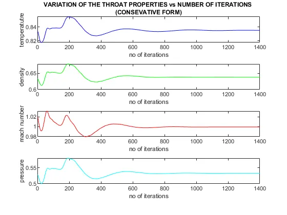
this are the variation of the throat properties with increase in the number of the grid points the solution is more smoother than previous results and . as the number of grid points increases the accuracy of the solution also increases. the oscillation become lesser
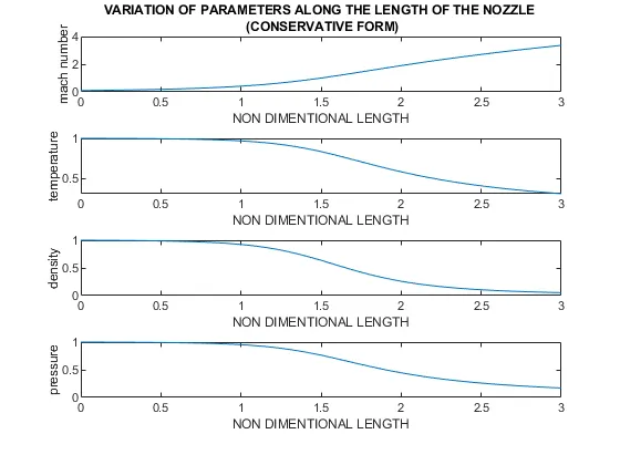
the mach number temperature, density,pressure, are the properties of the fluid which is flowing through the nozzle. as the length of the nozzle changes. during the convergent stage the fluid properties increase like temperature increases as the pressure increases, the and during the divergent stage the pressure decreases as the area increases and as the pressure decreases the temperature also decreases and the density also decreases as the area increases.
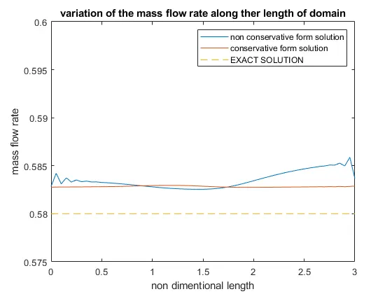
this graph shows the how our solution going to change if we change the number of the grid points as the number of grid points increases the solution going to give us more stable solution as the solution becomes more stable we are going close to the exact solution. when we compare this solution with the another solution with less fewer number of the grid points the difference between conservative and non conservative solution is more bu as we increase the number of grid points both are getting close to exact solution.