Week 5.2 - Literature review: ODE Stability

INTRODUCTION

Stability refers to the fact that errors at any point during the computation are not increased but rather attenuated as the computation advances. The sensitivity of a mathematical problem to changes in its input values is referred to as its condition. If the numerical approach changes the uncertainty of the input values abruptly, we call it numerically unstable computation.

APPROACHES TO STABILITY ANALYSIS METHODS:-

To solve a time-dependent differential equation, the explicit approach and implicit technique are numerical analysis methods.

The explicit method uses the current system status to calculate the system status in the future.

The implicit technique leverages the current and future system statuses to calculate the system status at a future time.

Consider the following differential equation y= F(x,t)

1. The explicit method expresses it as `y_(n+1) = y_n +hf(x_n,t_n)`. That is if we know the state at n we can calculate the state at n+1
2. When the implicit method express it as `y_(n+1)= y_n+hf(x_(n-1),t_(n-1))` that is it has a state on n+1 on the RHS

Code :

import numpy as np
import matplotlib.pyplot as plt 
import math

def explicit(time_total,dt):
	time=np.arange(0,time_total,dt) # The array construction technique arange() in NumPy is based on numerical ranges. It returns the reference to an instance of ndarray that has evenly spaced values.
	y=np.zeros(len(time)) #The numpy.zeros() method in Python creates a new array of the specified form and type, with the element's value set to 0.

	for i in range(0,len(time)):
		y[i]=y[i-1]+dt*(-1000*y[i-1] -math.exp(-time[i-1]));
	return[time,y]	

def implicit(time_total,dt):
	time=np.arange(0,time_total,dt)
	y=np.zeros(len(time))

	for i in range(0,len(time)):
		y[i]=(y[i-1]-math.exp(-time[i-1])*dt)/(1+1000*dt);
	return[time,y]	

time_total=0.1
dt=0.0005
	
time,y_exp=explicit(time_total,dt)
time,y_imp=implicit(time_total,dt)
plt.plot(time,y_exp)
plt.plot(time,y_imp)
plt.legend(('Explicit','Implicit'))
plt.grid(True)
titl=('Time_step:',dt)
plt.title(titl)
plt.show()

PLOTS:-

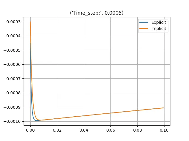
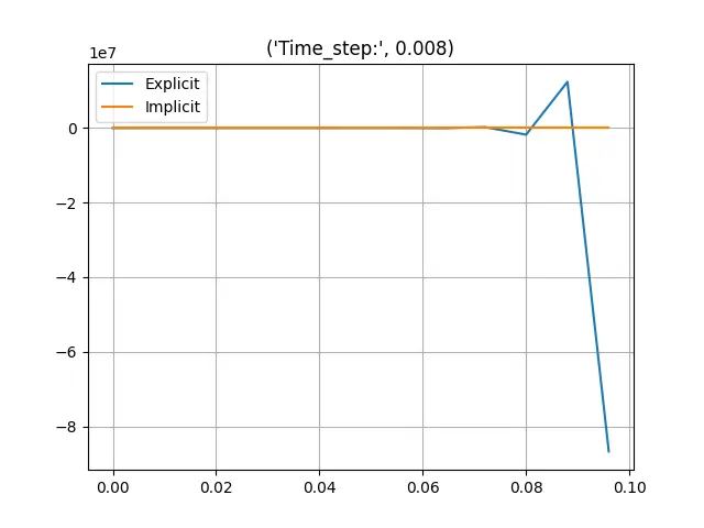
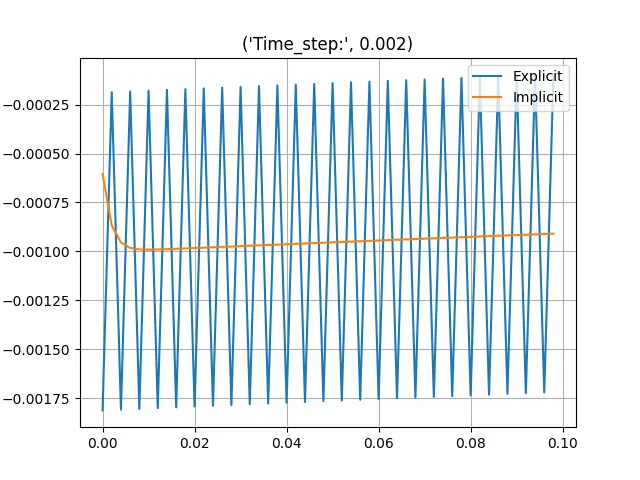
Both Implicit and Explicit schemes are performed on a function. Here the plots show how they score against each other.

Implicit v/s Explicit scheme at 0.0005s:-

Implicit v/s Explicit scheme at 0.008s:-

Implicit v/s Explicit scheme at 0.002s:-

RESULTS :

• When the number of subintervals is smaller or the value of sub-interval length is greater, the ODE becomes unstable in the case of an explicit scheme. At any number of subintervals, implicit schemes are stable. As we discretize and approximate in engineering simulations, there will always be some mistake; this error must be confined throughout the simulation. Before modeling any engineering problem, the stability requirement must be satisfied.For each issue in which there is an approximation, stability criteria may be obtained.

What is the point at which an ODE becomes unstable?

For each time step, an implicit solution comprises information collected by solving simultaneous equations for the entire grid. This is more computationally intensive, but it allows for bigger time steps and improved stability. The behavior of the solution when the time-step dt is raised is referred to as numerical stability. The approach is considered to be unconditionally stable if the solution behaves properly for arbitrarily high values of the time step. Explicit approaches, on the other hand, are always conditionally stable and become unstable as the dt (step) value grows. As a result, as dt grows, the ODE becomes unstable for this solution.

What is the impact of stability on engineering simulations?

When the solution of the precise differential equation is bounded, stability ensures that the numerical approach generates a bounded solution. If the solution isn't limited, it diverges, making it impossible to acquire a solution for a specific simulation.

Is it possible to derive stability criteria for all sorts of problems?

The term "neutrally stable" refers to a strategy in which mistakes remain constant as the calculations go. The implicit technique involves discretizing the differential equation in such a way that there are many unknowns on the LHS of the equation at the n+1 time level, but the terms on the RHS are known at the n time level. Implicit Schemes offer the advantage of not having to fulfill any stability criteria. They are inextricably stable. However, they are computationally costly since more storage space is required. As a result, we can solve any type of issue with an implicit scheme and suitable time step size selection. In general, there are two stability requirements that must be met Von Neumann stability analysis (also known as Fourier stability analysis) is a numerical analytic approach for determining the stability of finite difference schemes used to linear partial differential equations. The numerical error is decomposed using the Fourier transform.

If the system is represented by a matrix which is a recursive system, and if the eigenvalue > 1, that means if one initializes the corresponding eigenvector as input into the system (matrix), it will be amplified again and again without constraints, thus unstable. Similarly eigenvalues <= 1 are stable.