Week 7 - Auto ignition using Cantera

AIM: The aim of this challenge is to simulate the autoignition temperature for methane

OBJECTIVES :

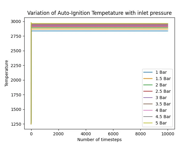
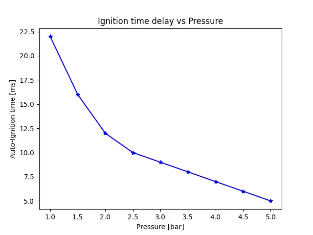
• With a constant temperature of 1250K and pressures ranging from 1 to 5 atm, the Auto Ignition time of methane varies.
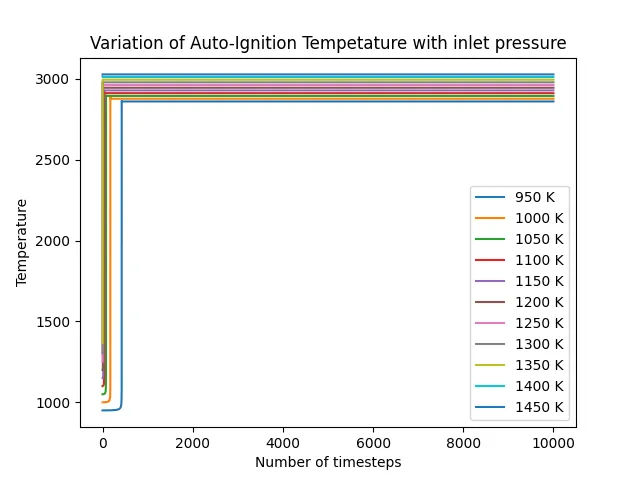
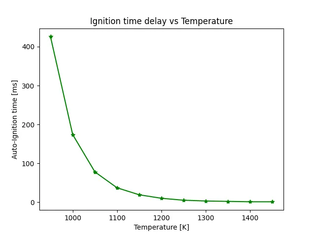
• With a constant pressure of 5 atm and temperatures ranging from 950K to 1450K, the Auto Ignition time of methane varies.
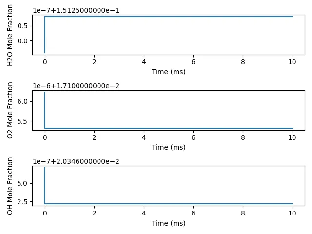
• Rate of change in the molar concentrations of the supplied elements "H20, 02, OH" over time

REACTORS NETWORK IN CANTERA :

The simplest kind of chemically reacting system is a Cantera Reactor (). It relates to a large thermodynamic control volume with uniform distribution of all state variables. The system is inherently unstable, in the sense that all states are time-dependent. Chemical processes, in particular, can cause transitory state shifts. Thermodynamic (but not chemical) equilibrium, on the other hand, is believed to exist throughout the reactor at all times.

Reactors can interact with their surroundings in a variety of ways:

• Expansion/compression work: The volume of the reactor may be modified by moving the reactor's walls, and expansion or compression work can be done by or on the reactor
• Heat transfer: To cross the reactor's boundaries, an arbitrary heat transfer rate can be specified
• The reactor can have several inlets and outputs for mass transfer. Arbitrary states can be established for the inlets. At the reactor's outputs, fluid in the reactor's present condition escapes.
• Surface interaction: The chemical processes in the reactor can be influenced by one or more walls. Mass transfer between the surface and the fluid may also be represented, thus it's not simply limited to catalytic processes.

All of these interactions don't have to be constant; they might change over time or as a function of state. Heat transfer, for example, can be treated as a function of the temperature difference between the reactor and the surrounding environment, or wall movement as a function of the pressure differential. On one or more walls, inlets, and outlets, the reactor's interactions with the environment are defined. Cantera can join reactors into a Reactor Network in addition to single reactors. A network of reactors can be linked together such that the contents of one reactor flow into another. Reactors can also communicate with one another and the outside world through walls that transfer heat or move to do tasks.

Governing Equations for Single Reactors :

The state variables for Canter's general reactor model are

• The mass of the reactor's contents (in kg)
• The reactor volume (in m3) (not a state variable for ConstPressureReactor () and IdealGasConstPressureReactor))
• A state variable describing the energy of the system, depending on the configuration (see Energy Conservation for further explanation):
  • General Reactor(): UU, the total internal energy of the contents of the reactor (in J)
  • ConstPressureReactor(): HH, the total enthalpy of the reactors contents (in J)
  • IdealGasReactor() and IdealGasConstPressureReactor(): TT, the temperature (in K)

• The mass fractions for each species (dimensionless)

Mass Conservation :

The total mass of the reactor's contents changes as a result of flow through the reactor's inlets and outlets, and production of homogeneous phase species on the reactor walls :

`frac(dm)(dt) = sum_(i n)dotm_(i n) - sum_(out)dotm_(out) + dotm_(wall)`

Species Conservation :

The rate at which species is generated through homogeneous phase reactions is `Vdotomega_kW_k`, and the total rate at which species is generated is:

`dotm_(k_(g en ) = Vdotomega_kW_k+dotm_(k_(wall))`

Applying Expanding the derivative on the left hand side , The equation for each homogeneous phase species is :

`mfrac(dY_k)(dt) = sum_(i n)dotm_(i n)(Y_(k_(i n )) - Y_k) + dotm_(k_(g en)) - Y_(k)dotm_(wall)`

Reactor Volume

The reactor volume changes as a function of time due to the motion of one or more walls:

`frac(dV)(dt) = sum_wf_wA_wv_W(t)`

For the ConstPressureReactor() and IdealGasConstPressureReactor), the volume is not a state variable but instead takes on whatever value is consistent with holding the pressure constant.

Energy Conservation

The solution of the energy equation can be enabled or disabled by changing the energy _enabled flag. It is enabled by default. The implemented formulation of the energy equation depends on which reactor model is used.

Standard Reactor

The equation for the total internal energy is found by writing the first law for an open system:

`frac(dU)(dt) = -p.frac(dV)(dt) - dotQ + sum_(i n)dotm_(i n)h_(i n) - h sum_(out)dotm_(out)`

Constant Pressure Reactor

For this reactor model, the pressure is held constant. The volume is not a state variable but instead takes on whatever value is consistent with holding the pressure constant. The total enthalpy replaces the total internal energy as a state variable. Using the definition of the total enthalpy:

`H = U + pV`

`frac(dH)(dt) = frac(dU)(dt) + pfrac(dV)(dt) + Vfrac(dp)(dt)`

by applying know values like `frac(dp)(dt) = 0`

`frac(dH)(dt) = -dotQ + sum_(i n) dotm_(i n)h_(i n) - h sum_(out)dotm_(out)`

Ideal Gas Reactor

In the case of the Ideal Gas Reactor Model, the reactor temperature is used instead of the total internal energy as a state variable.

Ideal Gas Constant Pressure Reactor

As for the Ideal Gas Reactor, we replace the total enthalpy as a state variable with the temperature by writing the total enthalpy in terms of the mass fractions and temperature:

`frac(dH)(dt) = h frac(dm)(dt)+ mc_pfrac(dT)(dt) +m sum_(k)h_k frac(dY_k)(dt)`

by applying theknown derivatives yields we get

`mc_pfrac(dT)(dt) = -dotQ - sum_(k) h_kdotm_(k_(g en)) + sum_(i n)dotm_(i n)(h_(i n) - sum_(k)h_kY_(k_(i n)))`

Code :

import matplotlib.pyplot as plt 
import cantera as ct 
import numpy as np 

''' 
The temperature of gas is assumed to be at 1250 k and then we write the start time and end time 
parameters in the subsequent lines of theprogram. We are saying the program to run the solution for 10
seconds with a time step of Ims or le-3 seconds. Now since the pressure is to be varied from 1 bar to 
5 bar, the linspace command defines 9 values of pressure. The for loop is used to execute the reactor 
network operations. Now when we define r, sim and states variables with the following statements, from 
these objects we are calling the respective classes of the created objects. Then we are appending the 
states object by defining the convergence loop of error 
'''

gas = ct.Solution('gri30.xml')
Pressure = np.linspace(1,5,9)
Temperature_intial = 1250
time_start = 0.0
time_end = 10.0
time_step = 1e-3
n = int((time_end - time_start)/time_step)
time_autoIgnition_Pressure = []
states1 =[]

for i in Pressure:
	gas.TPX = Temperature_intial, i*101325,{'CH4' : 1, 'O2':2, 'N2':7.52}
	Temperature_autoIgnition = 0
	time_autoIgnition = 0
	time = 0
	r = ct.IdealGasReactor(gas)
	sim = ct.ReactorNet([r])
	states = ct.SolutionArray(gas,extra = ['time_in_ms','t'])
	print('{:10s} {:10s} {:10s}'.format('t[s]','T[K]','P[Pa]'))

	for j in range(n) : 
		time += 1e-3
		sim.advance(time)
		states.append(r.thermo.state,time_in_ms = time*1e3,t=time)
		print('{:10.3e} {:10.3f} {:10.3f} '.format(sim.time,r.T,r.thermo.P))

	states1.append(states.T)
	
	for i in range(n):
		Temperature_error = states.T[i] - Temperature_intial - 400
		if Temperature_error >0:
			Temperature_autoIgnition = states.T[i]
			time_autoIgnition = states.time_in_ms[i]
			break
	time_autoIgnition_Pressure.append(time_autoIgnition)

states1 = np.array(states1)

for k in range(len(Pressure)):
	plt.figure(1)
	plt.plot(states1[k])
	plt.xlabel('Number of timesteps')
	plt.ylabel('Temperature')
	plt.title('Variation of Auto-Ignition Tempetature with inlet pressure')
	plt.legend(['1 Bar','1.5 Bar','2 Bar','2.5 Bar','3 Bar','3.5 Bar','4 Bar','4.5 Bar','5 Bar'])

plt.figure(2)
plt.plot(Pressure,time_autoIgnition_Pressure,'b-*')
plt.xlabel('Pressure [bar]')
plt.ylabel('Auto-Ignition time [ms]')
plt.title('Ignition time delay vs Pressure')
plt.show()

'''
The pressure of gas is assumed to be at 1.01325 bar and then we write the start time and end time 
parameters in the subsequent lines of the program. We are saying the program to run the solution for 10
seconds with a time step of Ims or le-3 seconds. Now since the temperature is to be varied from 950 K  
to 1450 K, the linspace command defines 11 values of pressure. The for loop is used to execute the 
reactor netwprk operations. Now When we define r, sim and states variables with the following statements, 
from these objects we are calling the respective classes of the created objects. Then we are appending 
the states object by defining the convergence loop of error.
'''

Temperature = np.linspace(950,1450,11)
time_autoIgnition_Temperature = []
states2 = []
for i in Temperature:
	gas.TPX = i, 5*101325,{'CH4' : 1, 'O2':2, 'N2':7.52}
	Temperature_autoIgnition = 0
	time_autoIgnition = 0
	time = 0
	r = ct.IdealGasReactor(gas)
	sim = ct.ReactorNet([r])
	states = ct.SolutionArray(gas,extra = ['time_in_ms','t'])
	print('{:10s} {:10s} {:10s}'.format('t[s]','T[K]','P[Pa]'))

	for j in range(n) : 
		time += 1e-3
		sim.advance(time)
		states.append(r.thermo.state,time_in_ms = time*1e3,t=time)
		print('{:10.3e} {:10.3f} {:10.3f} '.format(sim.time,r.T,r.thermo.P))

	states2.append(states.T)

	for j in range(n):
		Temperature_error = states.T[j] - Temperature_intial - 400
		if Temperature_error >0:
			Temperature_autoIgnition = states.T[j]
			time_autoIgnition = states.time_in_ms[j]
			break
	time_autoIgnition_Temperature.append(time_autoIgnition)

states2 = np.array(states2)

for m in range(len(Temperature)):
	plt.figure(3)
	plt.plot(states2[m])
	plt.xlabel('Number of timesteps')
	plt.ylabel('Temperature')
	plt.title('Variation of Auto-Ignition Tempetature with inlet pressure')
	plt.legend(['950 K','1000 K','1050 K','1100 K','1150 K','1200 K','1250 K','1300 K','1350 K','1400 K','1450 K'])

plt.figure(4)
plt.plot(Temperature,time_autoIgnition_Temperature,'g-*')
plt.xlabel('Temperature [K]')
plt.ylabel('Auto-Ignition time [ms]')
plt.title('Ignition time delay vs Temperature')
plt.show()

plt.figure(5)
plt.subplot(3,1,1)
plt.plot(states.t,states.X[:,gas.species_index('H2O')])
plt.xlabel('Time (ms)')
plt.ylabel('H2O Mole Fraction')
plt.subplot(3,1,2)
plt.plot(states.t,states.X[:,gas.species_index('O2')])
plt.xlabel('Time (ms)')
plt.ylabel('O2 Mole Fraction')
plt.subplot(3,1,3)
plt.plot(states.t,states.X[:,gas.species_index('OH')])
plt.xlabel('Time (ms)')
plt.ylabel('OH Mole Fraction')
plt.tight_layout()
plt.show()

'''
The pressure of gas is assumed to be at 1.01325 bar and then we write the start time and end time 
parameters in the subsequent lines of the program. We are saying the program to run the solution for 10
seconds with a time step of Ims or le-3 seconds. Now since the temperature is to be varied from 950 K bar 
to 1450 K, the linspace command defines 11 values of pressure. The for loop is used to execute the reactor 
network operations. Now when we define r, sim and states variables with the following statements, from 
these objects we are calling the respective classes of the created objects. Then we are appending the states
object by defining the convergence loop of error.
'''
AutoIgnition_Temperature = [500,1000]
states3 =[]
for i in AutoIgnition_Temperature:
	gas.TPX = i, 5*101325,{'CH4' : 1, 'O2':2, 'N2':7.52}
	r = ct.IdealGasReactor(gas)
	sim = ct.ReactorNet([r])
	time = 0
	states = ct.SolutionArray(gas)

	for n in range(1000):
		time += 1e-3
		sim.advance(time)
		states.append(r.thermo.state)

states3 = np.array(states.T)

plt.figure(6)
plt.plot(states3)
plt.xlabel('Number of timesteps')
plt.ylabel('Temperature')
plt.title('Temperature variation at 500 K & 1000 K')
plt.show()

Results :

Discussion :

1. The autoignition time of methane was studied at a constant temperature of 1250K and pressures ranging from 1 to 5 atm.

2. With a constant pressure of 5 atm and temperatures ranging from 950K to 1450K, the Auto Ignition time of methane varies. This research was carried out in the code's second case.

3. The rate of change in molar concentrations of the specified elements "H2O, 02, OH" over time was determined.

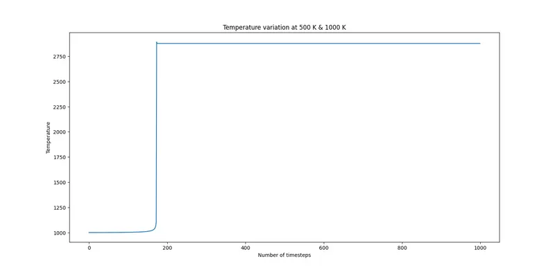
4. The impact of temperature for 500 K and 1000 K is displayed, with only 1000 K showing auto-ignition.