Week 3 - Adiabatic Flame Temperature calculation
Objectives of the Problem
- calculate adiabatic flame temperature,
- Adiabatic flame temperature variation with Equivalence ratio (In constant volume-chamber)
- Adiabatic flame temperature variation with Heat loss (In constant pressure-chamber)
- Adiabatic flame temperature variation with respect to Alkane, Alkene, Alkyne
- Adiabatic flame temperature variation with respect to a number of Carbon atom chains
Adiabatic Flame Temperature :
In the combustion process, the heat that is produced during the exothermic chemical reaction is released to the product and the temperature of the products are raised. There is no possibility for dissipation of heat in the surrounding, as there is no heat loss. As a result, the temperature of the product increases suddenly and produce a flame. This will heat the product gas in the flame region and the temperature rise will be maximum. This highest temperature is called AFT.
The temperature rise depends upon the amount of excess air used as an air-fuel ratio. The flame temperature has the highest value when using oxygen gas and decrease by using air. So exact stoichiometric air is required to supply for better results. With a too large amount of fuel, the flame temperature gets reduced. The flame temperature is determined from an energy balance.
Newton-Raphson Method
The Newton-Raphson method is one of the most widely used methods for root finding. It can be easily generalized to the problem of finding solutions to a system of non-linear equations, which is referred to as Newton's technique. Moreover, it can be shown that the technique is quadratically convergent as we approach the root.
Unlike the bisection and false position methods, the Newton-Raphson methods require only one initial value o, which we will refer to as the initial guess for the root.
To see how the N- method works, we can rewrite the function /lx) using a Taylor series expansion in `(x-x_o)`
`f(x) = f(x_o) + f(x_o)(x-x_o) + frac(1)(2)f'(x_o)(x-(x_o))^2 + ..... = 0`
where `f(x)`denotes the first derivative of `f(x)`with respect to x, `f'(x)`is the second derivative, and so forth. Now, suppose the initial guess is pretty close to the real root. Then `(x-x_o)` is small, and only the first few terms in the series are important to get an accurate estimate of the true root, given `x_o`. By truncating the series at the second term (linear in x), we obtain the N-R iteration formula for getting a better estimate of the true root:
`x_1 = x_o -frac(f(x_o))(f'(x_o))`
Thus the N-R method finds the tangent to the function `f(x)` at `x=x_o` and extrapolates it to intersect the x-axis to get `x_1`. This point of the intersection is taken as the new approximation to the root and the procedure is repeated until convergence is obtained whenever possible.
Mathematically, given the value of `x=x_i` at the end of the ith iteration, we obtain `x_(i+1)` as
`x_(i+1) = x_i - frac(f(x_i))(f'(x_i)`
Graphically we can represent this method is as:
THE CONCEPT OF AIR-FUEL MIXTURE:
STOICHIOMETRIC COMBUSTION:
The air-fuel ratio for complete combustion is called the stoichiometric air-fuel ratio.
LEAN COMBUSTION:
If the amount of air is more than fuel for complete combustion. This is called lean combustion.
RICH MIXTURE:
If the amount of fuel is more than air for complete combustion. This is called rich combustion.
EQUIVALENCE RATIO:
The fuel-air equivalence ratio (phi) of a system is defined as the ratio of the fuel to oxidizer ratio to the stoichiometric fuel to oxidiser
ratio.
`phi` = Actual Air Fuel Ratio / statiometric Air Fuel Ratio
`phi` = `frac(frac(F)(A))(frac(F)(A))_(stOiChiometric)`
`phi`< 1, lean combustion
`phi`= 1. stoichiometric combustion.
`phi` > 1, rich combustion.
GENERAL EQUATION FOR ANY HYDROCARBON COMBUSTION:
`C_xH_y + [x+(y/4)](O_2+3.76N_2) to xCO_2 + (y/2)H_2O + 3.76[x+(y/4)]N_2`
CHEMICAL REACTION FOR COMBUSTION OF METHANE :
STOICHIOMETRIC COMBUSTION :
`CH_4 + 2(O_2+3.76N_2) to CO_2 +2H_2O +7.52N_2`
EQUIVALENCE RATIO COMBUSTION :
`CH_4 + (2/phi)(O_2+3.76N_2) to CO_2 +y2H_2O`+Products
LEAN COMBUSTION :
`CH_4 + (2/phi)(O_2+3.76N_2) to CO_2 +2H_2O +((2/phi)-2)O_2 +(7.52/phi)N_2`
RICH COMBUSTION :
`CH_4 + (2/phi)(O_2+3.76N_2) to (4/phi-3)CO_2 +2H_2O +(4-4/phi)CO +(7.52/phi)N_2`
Case 1 :
Adiabatic flame temperature variation with Equivalence ratio (In constant volume-chamber) Assume that methane is contained in a constant volume chamber. Write a program in Python to plot the effect of equivalence ratio on the final adiabatic flame temperature. Compare the results with Cantera. Assume that N2 is present.
'''
PYTHON PROGRAMM TO SOLVE THE EFFECT OF EQUIVLENCE RATIO ON AFT OF CH4 FOR CONSTANT VOLUME CHAMBER
GENERAL EQUATION FOR ANY HYDROCARBON COMBUSTION:
`C_xH_y + [x+(y/4)](O_2+3.76N_2) to xCO_2 + (y/2)H_2O + 3.76[x+(y/4)]N_2`

CHEMICAL REACTION FOR COMBUSTION OF METHANE :

STOICHIOMETRIC COMBUSTION :

`CH_4 + 2(O_2+3.76N_2) to CO_2 +2H_2O +7.52N_2`

EQUIVALENCE RATIO COMBUSTION :

`CH_4 + (2/phi)(O_2+3.76N_2) to CO_2 +y2H_2O + products`

LEAN COMBUSTION :

`CH_4 + (2/phi)(O_2+3.76N_2) to CO_2 +2H_2O +((2/phi)-2)O_2 +(7.52/phi)N_2`

RICH COMBUSTION :
`CH_4 + (2/phi)(O_2+3.76N_2) to (4/phi-3)CO_2 +2H_2O +(4-4/phi)CO +(7.52/phi)N_2`

CODE WRITTEN BY : CHALUMURU MANAS
'''

import numpy as np
import matplotlib.pyplot as plt

def h(Temp,coeff):

	R = 8.314       #J/mol-K
	a1 = coeff[0]
	a2 = coeff[1]
	a3 = coeff[2]
	a4 = coeff[3]
	a5 = coeff[4]
	a6 = coeff[5]
	a7 = coeff[6]

	return (a1 + a2*(Temp/2) + a3*(pow(Temp,2)/3) + a4*(pow(Temp,3)/4) + a5*(pow(Temp,4)/5) + a6/Temp) * R * Temp

#Low Temperature coefficients of the Reactents at STP Condition
CH4_coeffs_Low_Temp = [5.14987613E+00,-1.36709788E-02,4.91800599E-05,-4.84743026E-08,1.66693956E-11,-1.02466476E+04,-4.64130376E+00 ]
O2_coeffs_Low_Temp = [3.78245636E+00,-2.99673416E-03,9.84730201E-06,-9.68129509E-09,3.24372837E-12,-1.06394356E+03,3.65767573E+00 ]
N2_coeffs_Low_Temp = [0.03298677E+02,0.14082404E-02,-0.03963222E-04,0.05641515E-07,-0.02444854E-10,-0.10208999E+04,0.03950372E+02 ]

#High Temperature coefficients of the Products
N2_coeffs_High_Temp = [0.02926640E+02,0.14879768E-02,-0.05684760E-05,0.10097038E-09,-0.06753351E-13,-0.09227977E+04,0.05980528E+02 ]
CO2_coeffs_High_Temp = [3.85746029E+00,4.41437026E-03,-2.21481404E-06,5.23490188E-10,-4.72084164E-14,-4.87591660E+04,2.27163806E+00 ]
H2O_coeffs_High_Temp = [3.03399249E+00,2.17691804E-03,-1.64072518E-07,-9.70419870E-11,1.68200992E-14,-3.00042971E+04,4.96677010E+00 ]
CO_coeffs_High_Temp = [2.71518561E+00,2.06252743E-03,-9.98825771E-07,2.30053008E-10,-2.03647716E-14,-1.41518724E+04,7.81868772E+00 ]
O2_coeffs_High_Temp = [3.28253784E+00,1.48308754E-03,-7.57966669E-07,2.09470555E-10,-2.16717794E-14,-1.08845772E+03,5.45323129E+00 ]


#calculating Enthalpy of reactants and products
def f(Temp,psi):

	Temp_stp = 298.15  #k
	R = 8.314  #J/mol-K

	h_CH4_Reactents = h(Temp_stp,CH4_coeffs_Low_Temp)	#J/mol-K
	h_O2_Reactents = h(Temp_stp,O2_coeffs_Low_Temp)		#J/mol-K
	h_N2_Reactents = h(Temp_stp,N2_coeffs_Low_Temp)		#J/mol-K

	h_CO2_Products = h(Temp,CO2_coeffs_High_Temp)		#J/mol-K
	h_H2O_Products = h(Temp,H2O_coeffs_High_Temp)		#J/mol-K
	h_O2_Products = h(Temp,O2_coeffs_High_Temp)			#J/mol-K
	h_N2_Products = h(Temp,N2_coeffs_High_Temp)			#J/mol-K
	h_CO_Products = h(Temp,CO_coeffs_High_Temp)			#J/mol-K

	if psi>1:
		H_Reactents =  h_CH4_Reactents + (2/psi)*(h_O2_Reactents) + (7.52/psi)*(h_N2_Reactents)
		H_Products = ((4/psi)-3) * h_CO2_Products + 2*h_H2O_Products + (4-(4/psi))*h_CO_Products + (7.52/psi)*h_N2_Products
		N_Reactents = (1+(2/psi)+(7.52/psi))*R*Temp_stp
		N_Products = (((4/psi)-3)+2+(4-(4/psi)+(7.52/psi))) *R*Temp
	else:
		H_Reactents =  h_CH4_Reactents + (2/psi)*(h_O2_Reactents) + (7.52/psi)*(h_N2_Reactents)
		H_Products = h_CO2_Products + 2*h_H2O_Products + ((2/psi)-2)*h_O2_Products + (7.52/psi)*h_N2_Products
		N_Reactents = (1+(2/psi)+(7.52/psi)) * R *Temp_stp
		N_Products = (1+2+(7.52/psi) + (2/psi)-2)*R*Temp


	return H_Products - H_Reactents - (N_Products - N_Reactents)


def fprime(Temp,psi):
	return (f(Temp+1e-6,psi) - f(Temp,psi))/(1e-6)


Temp_guess = 1500  #K
tol = 1e-3
Iteration = 0
alpha = 0.2
psi = np.linspace(0.1,2,100)

Temp_aft = []

for i in psi:
	while (abs(f(Temp_guess,i))>tol):
			Temp_guess = Temp_guess-(alpha*((f(Temp_guess,i))/(fprime(Temp_guess,i))))
			Iteration=Iteration+1
	Temp_aft.append(Temp_guess)


import cantera as ct
gas = ct.Solution('gri30.xml')

Temp_aft_cantera = []

for i in range(0,len(psi)):
	#Total_mole = 1 + 2/psi[i] + 7.52/psi[i]
	Mole_Fraction_CH4 = 1
	Mole_Fraction_O2 = (2/psi[i])
	Mole_Fraction_N2 = (7.52/psi[i])

	gas.TPX = 298.15,101325,{'CH4' : Mole_Fraction_CH4 , 'O2' : Mole_Fraction_O2 , 'N2' : Mole_Fraction_N2}
	gas.equilibrate('UV','auto')
	Temp_aft_cantera.append(gas.T)

Equivalence_ratio = psi
plt.plot(Equivalence_ratio,Temp_aft,color = 'blue')
plt.plot(Equivalence_ratio,Temp_aft_cantera,color = 'red')
plt.xlabel('Equivalence Ratio')
plt.ylabel('Adiabaatic Flame Temperature(K)')
plt.grid()
plt.title('Effect of Equivalence ratio on the AFT')
plt.legend(['Python','Cantera'])
plt.show()
Output :
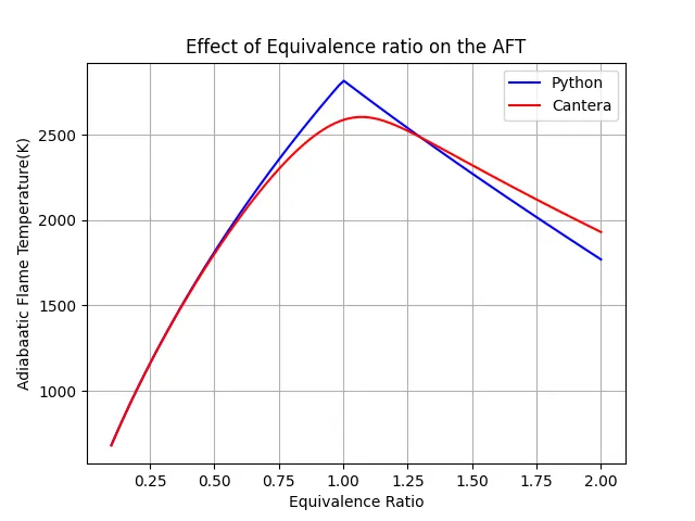
Discussion :
1. We can observe here, we will get the high adiabatic flame temperature at `phi`=1 using python but if we take a look at the curve of AFT using Cantera high AFT is in between the equivalence ratio of 1 to 1.25.
2. No of participating species at the product side using python is less compared to Cantera hence we get a somewhat high adiabatic flame temperature than that of CANTERA. In CANTERA, since it is a standard chemical kinetics library the no of species will be more at the product side.
3. Practically we operate at an equivalence ratio of 0.5 to 1.5.
4. Cantera gives slightly more value of AFT after the equivalence ratio increases more than 1.3 approximately.
Case 2:
Adiabatic flame temperature variation with Heat loss (In constant pressure chamber): Consider a constant pressure reactor with heat loss. The reactor is initially set at STP conditions. The heat loss should be input in your program and must be a fraction of the "maximum possible heat loss". You will control heat loss using a variable called H_loss. For example, H_loss = 0.5 would mean a heat loss that is equal to 50% of the maximum possible heat loss. The fuel type can be a general hydrocarbon of the form CxHy. Phi and lambda = 1.0. Find the AFT of CH4 with H loss = 0.35
import numpy as np
import matplotlib.pyplot as plt
import math


def h(T,coeff):

	R = 8.314
	a1 = coeff[0]
	a2 = coeff[1]
	a3 = coeff[2]
	a4 = coeff[3]
	a5 = coeff[4]
	a6 = coeff[5]
	a7 = coeff[6]

	return (a1 + a2*(T/2) + a3*(pow(T,2)/3) + a4*(pow(T,3)/4) + a5*(pow(T,4)/5) + a6/T) * R * T


CH4_coeffs_Low_Temp = [5.14987613E+00,-1.36709788E-02,4.91800599E-05,-4.84743026E-08,1.66693956E-11,-1.02466476E+04,-4.64130376E+00 ]
O2_coeffs_Low_Temp = [3.78245636E+00,-2.99673416E-03,9.84730201E-06,-9.68129509E-09,3.24372837E-12,-1.06394356E+03,3.65767573E+00 ]
N2_coeffs_Low_Temp = [0.03298677E+02,0.14082404E-02,-0.03963222E-04,0.05641515E-07,-0.02444854E-10,-0.10208999E+04,0.03950372E+02 ]
N2_coeffs_High_Temp = [0.02926640E+02,0.14879768E-02,-0.05684760E-05,0.10097038E-09,-0.06753351E-13,-0.09227977E+04,0.05980528E+02 ]
CO2_coeffs_High_Temp = [3.85746029E+00,4.41437026E-03,-2.21481404E-06,5.23490188E-10,-4.72084164E-14,-4.87591660E+04,2.27163806E+00 ]
H2O_coeffs_High_Temp = [3.03399249E+00,2.17691804E-03,-1.64072518E-07,-9.70419870E-11,1.68200992E-14,-3.00042971E+04,4.96677010E+00 ]
CO_coeffs_High_Temp = [2.71518561E+00,2.06252743E-03,-9.98825771E-07,2.30053008E-10,-2.03647716E-14,-1.41518724E+04,7.81868772E+00 ]
O2_coeffs_High_Temp = [3.28253784E+00,1.48308754E-03,-7.57966669E-07,2.09470555E-10,-2.16717794E-14,-1.08845772E+03,5.45323129E+00 ]


T_stp = 298.15
Heat_Supplied = 802000
Heat_Loss = np.linspace(0,1,21)
def f(T,Heat_Loss):

	h_CH4_Reactents = h(T_stp,CH4_coeffs_Low_Temp)
	h_O2_Reactents = h(T_stp,O2_coeffs_Low_Temp)
	h_N2_Reactents = h(T_stp,N2_coeffs_Low_Temp)

	h_CO2_Products = h(T,CO2_coeffs_High_Temp)
	h_H2O_Products = h(T,H2O_coeffs_High_Temp)
	h_O2_Products = h(T,O2_coeffs_High_Temp)
	h_N2_Products = h(T,N2_coeffs_High_Temp)
	h_CO_Products = h(T,CO_coeffs_High_Temp)

	H_Products = h_CO2_Products + 2*h_H2O_Products + 7.52*h_N2_Products
	H_Reactents = h_CH4_Reactents + 2*h_O2_Reactents + 7.52*h_N2_Reactents

	print (H_Products)
	print (H_Reactents)


	return H_Products - H_Reactents + (Heat_Loss*Heat_Supplied)


def fprime(T,Heat_Loss):
	return (f(T+1e-6,Heat_Loss) - f(T,Heat_Loss))/(1e-6)


T_guess = 1500
tol = 1e-3
ct = 0
alpha = 0.8
Temp = []

for i in Heat_Loss:
	while (abs(f(T_guess,i))>tol):
		T_guess = T_guess-(alpha*((f(T_guess,i))/(fprime(T_guess,i))))
		ct=ct+1
	Temp.append(T_guess)

print(Temp)
Temp_loss = Temp[7]
print(Temp_loss)

plt.plot(Heat_Loss,Temp,color = 'red')
plt.plot(Heat_Loss[7],Temp[7],'*',label = 'Heat Loss = 0.35', color = 'black' )
plt.xlabel('Heat Loss Coefficients')
plt.ylabel('Adiabaatic Flame Temperature(K) Heat Loss')
plt.title('Effect of Heat Loss Factor on AFT')
plt.grid()
plt.show()
Output :
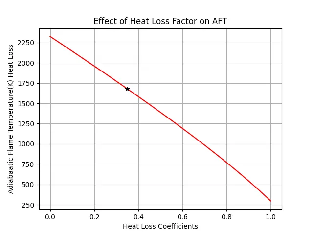
Discussion :
- AFT varies linearly with a heat loss coefficient
- AFT value at 0.35 heat loss coefficient is 1678.83k
Case 3:
Adiabatic flame temperature variation with respect to Alkane, Alkene, Alkyne: Test it only for Alk-ane, -ene and -ye variants of 2 Carbon atom chain and plot a trend. The provided therm.dat might not contain data for other alkanes, alkynes, and alkenes (in that case use Cantera). Assume no heat loss.
import numpy as np
import matplotlib.pyplot as plt
import cantera as ct

def h(T,coeff):

	R = 8.314
	a1 = coeff[0]
	a2 = coeff[1]
	a3 = coeff[2]
	a4 = coeff[3]
	a5 = coeff[4]
	a6 = coeff[5]
	a7 = coeff[6]

	return (a1 + a2*(T/2) + a3*(pow(T,2)/3) + a4*(pow(T,3)/4) + a5*(pow(T,4)/5) + a6/T) * R * T


C2H6_coeffs_Low_Temp = [1.07188150E+00,2.16852677E-02,-1.00256067E-05,2.21412001E-09,-1.90002890E-13,-1.14263932E+04,1.51156107E+01]
C2H4_coeffs_Low_Temp = [2.03611116E+00,1.46454151E-02,-6.71077915E-06,1.47222923E-09,-1.25706061E-13,4.93988614E+03,1.03053693E+01 ]
C2H2_coeffs_Low_Temp = [4.14756964E+00,5.96166664E-03,-2.37294852E-06,4.67412171E-10,-3.61235213E-14,2.59359992E+04,-1.23028121E+00]
O2_coeffs_Low_Temp = [3.78245636E+00,-2.99673416E-03,9.84730201E-06,-9.68129509E-09,3.24372837E-12,-1.06394356E+03,3.65767573E+00 ]
N2_coeffs_Low_Temp = [0.03298677E+02,0.14082404E-02,-0.03963222E-04,0.05641515E-07,-0.02444854E-10,-0.10208999E+04,0.03950372E+02 ]
N2_coeffs_High_Temp = [0.02926640E+02,0.14879768E-02,-0.05684760E-05,0.10097038E-09,-0.06753351E-13,-0.09227977E+04,0.05980528E+02 ]
CO2_coeffs_High_Temp = [3.85746029E+00,4.41437026E-03,-2.21481404E-06,5.23490188E-10,-4.72084164E-14,-4.87591660E+04,2.27163806E+00 ]
H2O_coeffs_High_Temp = [3.03399249E+00,2.17691804E-03,-1.64072518E-07,-9.70419870E-11,1.68200992E-14,-3.00042971E+04,4.96677010E+00 ]
CO_coeffs_High_Temp = [2.71518561E+00,2.06252743E-03,-9.98825771E-07,2.30053008E-10,-2.03647716E-14,-1.41518724E+04,7.81868772E+00 ]
O2_coeffs_High_Temp = [3.28253784E+00,1.48308754E-03,-7.57966669E-07,2.09470555E-10,-2.16717794E-14,-1.08845772E+03,5.45323129E+00 ]


def f_Alkanes(T):

	T_stp = 298.15
	Heat_Loss = 0.35
	LHV = 1428275

	h_C2H6_Reactents = h(T_stp,C2H6_coeffs_Low_Temp)
	h_O2_Reactents = h(T_stp,O2_coeffs_Low_Temp)
	h_N2_Reactents = h(T_stp,N2_coeffs_Low_Temp)

	h_CO2_Products = h(T,CO2_coeffs_High_Temp)
	h_H2O_Products = h(T,H2O_coeffs_High_Temp)
	h_N2_Products = h(T,N2_coeffs_High_Temp)

	H_Products = 2*h_CO2_Products + 3*h_H2O_Products + (3.5*3.76)*h_N2_Products
	H_Reactents = h_C2H6_Reactents + 3.5*h_O2_Reactents + (3.5*3.76)*h_N2_Reactents

	print (H_Products)
	print (H_Reactents)

	Loss = Heat_Loss * LHV
	return H_Products - H_Reactents + Loss


def fprime_Alkanes(T):
	return (f_Alkanes(T+1e-6) - f_Alkanes(T))/(1e-6)


def f_Alkenes(T):

	T_stp = 298.15
	Heat_Loss = 0.35
	LHV = 1428275

	h_C2H4_Reactents = h(T_stp,C2H4_coeffs_Low_Temp)
	h_O2_Reactents = h(T_stp,O2_coeffs_Low_Temp)
	h_N2_Reactents = h(T_stp,N2_coeffs_Low_Temp)

	h_CO2_Products = h(T,CO2_coeffs_High_Temp)
	h_H2O_Products = h(T,H2O_coeffs_High_Temp)
	h_N2_Products = h(T,N2_coeffs_High_Temp)

	H_Products = 2*h_CO2_Products + 2*h_H2O_Products + (3*3.76)*h_N2_Products
	H_Reactents = h_C2H4_Reactents + 3*h_O2_Reactents + (3*3.76)*h_N2_Reactents

	print (H_Products)
	print (H_Reactents)

	Loss = Heat_Loss * LHV
	return H_Products - H_Reactents + Loss


def fprime_Alkenes(T):
	return (f_Alkenes(T+1e-6) - f_Alkenes(T))/(1e-6)


def f_Alkynes(T):

	T_stp = 298.15
	Heat_Loss = 0.35
	LHV = 1258020

	h_C2H2_Reactents = h(T_stp,C2H2_coeffs_Low_Temp)
	h_O2_Reactents = h(T_stp,O2_coeffs_Low_Temp)
	h_N2_Reactents = h(T_stp,N2_coeffs_Low_Temp)

	h_CO2_Products = h(T,CO2_coeffs_High_Temp)
	h_H2O_Products = h(T,H2O_coeffs_High_Temp)
	h_N2_Products = h(T,N2_coeffs_High_Temp)

	H_Products = 2*h_CO2_Products + h_H2O_Products + (2.5*3.76)*h_N2_Products
	H_Reactents = h_C2H2_Reactents + 2.5*h_O2_Reactents + (2.5*3.76)*h_N2_Reactents

	print (H_Products)
	print (H_Reactents)

	Loss = Heat_Loss * LHV
	return H_Products - H_Reactents + Loss


def fprime_Alkynes(T):
	return (f_Alkynes(T+1e-6) - f_Alkynes(T))/(1e-6)


T_Alkanes_guess = 1500
tol = 1e-3
Iterations_Alkanes = 0
alpha = 0.2
T_aft = []

while (abs(f_Alkanes(T_Alkanes_guess))>tol):
	T_Alkanes_guess = T_Alkanes_guess-(alpha*((f_Alkanes(T_Alkanes_guess))/(fprime_Alkanes(T_Alkanes_guess))))
	Iterations_Alkanes =Iterations_Alkanes +1
T_aft.append(T_Alkanes_guess)

T_Alkenes_guess = 1500
tol = 1e-3
Iterations_Alkenes = 0
alpha = 0.2
while (abs(f_Alkenes(T_Alkenes_guess))>tol):
	T_Alkenes_guess = T_Alkenes_guess-(alpha*((f_Alkenes(T_Alkenes_guess))/(fprime_Alkenes(T_Alkenes_guess))))
	Iterations_Alkenes=Iterations_Alkenes+1
T_aft.append(T_Alkenes_guess)

T_Alkynes_guess = 1500
tol = 1e-3
Iterations_Alkynes = 0
alpha = 0.2
while (abs(f_Alkynes(T_Alkynes_guess))>tol):
	T_Alkynes_guess = T_Alkynes_guess-(alpha*((f_Alkynes(T_Alkynes_guess))/(fprime_Alkynes(T_Alkynes_guess))))
	Iterations_Alkenes=Iterations_Alkenes+1
T_aft.append(T_Alkynes_guess)


gas =ct.Solution('gri30.xml')


gas.TPX = 298.15,101325,{'C2H6':1,'O2':3.5,'N2':13.16}
gas.equilibrate('HP','auto')
Temp_alkane= gas.T

gas.TPX = 298.15,101325,{'C2H4':1,'O2':3,'N2':11.28}
gas.equilibrate('HP','auto')
Temp_alkene=gas.T

gas.TPX = 298.15,101325,{'C2H2':1,'O2':2.5,'N2':9.4}
gas.equilibrate('HP','auto')
Temp_alkyne=gas.T

Temp = [Temp_alkane,Temp_alkene,Temp_alkyne]

plt.figure(1)
fuel=['Ethane($C_2H_6$)','Ethene($C_2H_4$)','Ethyne($C_2H_2$)']
print(T_aft)
plt.bar(fuel,T_aft)
plt.xlabel('Type Of Fuel')
plt.ylabel('Adiabatic Flame Temperature(K)')
plt.title('effect of Type of Fuel on AFT')
plt.show()

plt.figure(2)
fuel=['Ethane($C_2H_6$)','Ethene($C_2H_4$)','Ethyne($C_2H_2$)']
print(Temp)
plt.bar(fuel,Temp)
plt.xlabel('Type Of Fuel')
plt.ylabel('Adiabatic Flame Temperature(K)')
plt.title('effect of Type of Fuel on AFT (Cantera)')
plt.show()
Output:
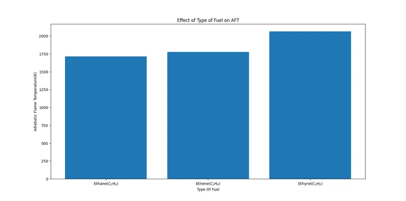
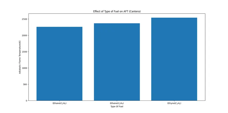
Discussion :
1. We can observe here is that lowering the hydrogen atoms leads to increasing the AFT of CH4 because it will produce less H2O on the product side.
2. In Cantera, for all fuel types, AFT is lower because of an increase in species at the product's side.
Case 4 :
Adiabatic flame temperature variation with respect to a number of Carbon atom chains :
For a general alkane, plot the effect of the number of carbon atoms (from 1 to 3) on the final temperature. Assume no heat loss.
import numpy as np
import matplotlib.pyplot as plt
import cantera as ct

def h(T,coeff):

	R = 8.314
	a1 = coeff[0]
	a2 = coeff[1]
	a3 = coeff[2]
	a4 = coeff[3]
	a5 = coeff[4]
	a6 = coeff[5]
	a7 = coeff[6]

	return (a1 + a2*(T/2) + a3*(pow(T,2)/3) + a4*(pow(T,3)/4) + a5*(pow(T,4)/5) + a6/T) * R * T

CH4_coeffs_Low_Temp = [7.48514950E-02,1.33909467E-02,-5.73285809E-06,1.22292535E-09,-1.01815230E-13,-9.46834459E+03,1.84373180E+01]
C3H8_coeffs_Low_Temp = [0.75341368E+01,0.18872239E-01,-0.62718491E-05,0.91475649E-09,-0.47838069E-13,-0.16467516E+05,-0.17892349E+02]
C2H6_coeffs_Low_Temp = [1.07188150E+00,2.16852677E-02,-1.00256067E-05,2.21412001E-09,-1.90002890E-13,-1.14263932E+04,1.51156107E+01]
C2H4_coeffs_Low_Temp = [2.03611116E+00,1.46454151E-02,-6.71077915E-06,1.47222923E-09,-1.25706061E-13,4.93988614E+03,1.03053693E+01 ]
C2H2_coeffs_Low_Temp = [4.14756964E+00,5.96166664E-03,-2.37294852E-06,4.67412171E-10,-3.61235213E-14,2.59359992E+04,-1.23028121E+00]
O2_coeffs_Low_Temp = [3.78245636E+00,-2.99673416E-03,9.84730201E-06,-9.68129509E-09,3.24372837E-12,-1.06394356E+03,3.65767573E+00 ]
N2_coeffs_Low_Temp = [0.03298677E+02,0.14082404E-02,-0.03963222E-04,0.05641515E-07,-0.02444854E-10,-0.10208999E+04,0.03950372E+02 ]
N2_coeffs_High_Temp = [0.02926640E+02,0.14879768E-02,-0.05684760E-05,0.10097038E-09,-0.06753351E-13,-0.09227977E+04,0.05980528E+02 ]
CO2_coeffs_High_Temp = [3.85746029E+00,4.41437026E-03,-2.21481404E-06,5.23490188E-10,-4.72084164E-14,-4.87591660E+04,2.27163806E+00 ]
H2O_coeffs_High_Temp = [3.03399249E+00,2.17691804E-03,-1.64072518E-07,-9.70419870E-11,1.68200992E-14,-3.00042971E+04,4.96677010E+00 ]
CO_coeffs_High_Temp = [2.71518561E+00,2.06252743E-03,-9.98825771E-07,2.30053008E-10,-2.03647716E-14,-1.41518724E+04,7.81868772E+00 ]
O2_coeffs_High_Temp = [3.28253784E+00,1.48308754E-03,-7.57966669E-07,2.09470555E-10,-2.16717794E-14,-1.08845772E+03,5.45323129E+00 ]


def f_Methane(T):

	T_stp = 298.15

	h_CH4_Reactents = h(T_stp,CH4_coeffs_Low_Temp)
	h_O2_Reactents = h(T_stp,O2_coeffs_Low_Temp)
	h_N2_Reactents = h(T_stp,N2_coeffs_Low_Temp)

	h_CO2_Products = h(T,CO2_coeffs_High_Temp)
	h_H2O_Products = h(T,H2O_coeffs_High_Temp)
	h_N2_Products = h(T,N2_coeffs_High_Temp)

	H_Products = h_CO2_Products + 2*h_H2O_Products + (2*3.76)*h_N2_Products
	H_Reactents = h_CH4_Reactents + 2*h_O2_Reactents + (2*3.76)*h_N2_Reactents

	print (H_Products)
	print (H_Reactents)

	return H_Products - H_Reactents


def fprime_Methane(T):
	return (f_Methane(T+1e-6) - f_Methane(T))/(1e-6)


def f_Ethane(T):

	T_stp = 298.15

	h_C2H6_Reactents = h(T_stp,C2H6_coeffs_Low_Temp)
	h_O2_Reactents = h(T_stp,O2_coeffs_Low_Temp)
	h_N2_Reactents = h(T_stp,N2_coeffs_Low_Temp)

	h_CO2_Products = h(T,CO2_coeffs_High_Temp)
	h_H2O_Products = h(T,H2O_coeffs_High_Temp)
	h_N2_Products = h(T,N2_coeffs_High_Temp)

	H_Products = 2*h_CO2_Products + 3*h_H2O_Products + (3.5*3.76)*h_N2_Products
	H_Reactents = h_C2H6_Reactents + 3.5*h_O2_Reactents + (3.5*3.76)*h_N2_Reactents

	print (H_Products)
	print (H_Reactents)

	return H_Products - H_Reactents


def fprime_Ethane(T):
	return (f_Ethane(T+1e-6) - f_Ethane(T))/(1e-6)


def f_Propane(T):

	T_stp = 298.15

	h_C3H8_Reactents = h(T_stp,C3H8_coeffs_Low_Temp)
	h_O2_Reactents = h(T_stp,O2_coeffs_Low_Temp)
	h_N2_Reactents = h(T_stp,N2_coeffs_Low_Temp)

	h_CO2_Products = h(T,CO2_coeffs_High_Temp)
	h_H2O_Products = h(T,H2O_coeffs_High_Temp)
	h_N2_Products = h(T,N2_coeffs_High_Temp)

	H_Products = 3*h_CO2_Products + 4*h_H2O_Products + (5*3.76)*h_N2_Products
	H_Reactents = h_C3H8_Reactents + 5*h_O2_Reactents + (5*3.76)*h_N2_Reactents

	print (H_Products)
	print (H_Reactents)

	return H_Products - H_Reactents


def fprime_Propane(T):
	return (f_Propane(T+1e-6) - f_Propane(T))/(1e-6)


T_Methane_guess = 1500
tol = 1e-3
Iterations_Methane = 0
alpha = 0.2
T_aft = []

while (abs(f_Methane(T_Methane_guess))>tol):
	T_Methane_guess = T_Methane_guess-(alpha*((f_Methane(T_Methane_guess))/(fprime_Methane(T_Methane_guess))))
	Iterations_Methane =Iterations_Methane +1
T_aft.append(T_Methane_guess)

T_Ethane_guess = 1500
tol = 1e-3
Iterations_Ethane = 0
alpha = 0.2
while (abs(f_Ethane(T_Ethane_guess))>tol):
	T_Ethane_guess = T_Ethane_guess-(alpha*((f_Ethane(T_Ethane_guess))/(fprime_Ethane(T_Ethane_guess))))
	Iterations_Ethane=Iterations_Ethane+1
T_aft.append(T_Ethane_guess)

T_Propane_guess = 1500
tol = 1e-3
Iterations_Propane = 0
alpha = 0.2
while (abs(f_Propane(T_Propane_guess))>tol):
	T_Propane_guess = T_Propane_guess-(alpha*((f_Propane(T_Propane_guess))/(fprime_Propane(T_Propane_guess))))
	Iterations_Propane=Iterations_Propane+1
T_aft.append(T_Propane_guess)


fuel=['Methane($CH_4$)','Ethane($C_2H_6$)','Propane($C_3H_8$']
print(T_aft)
plt.bar(fuel,T_aft)
plt.xlabel('Type Of Fuel')
plt.ylabel('Adiabatic Flame Temperature(K)')
plt.title('Effect Of carbon atoms on thr AFT')
plt.show()
Output :
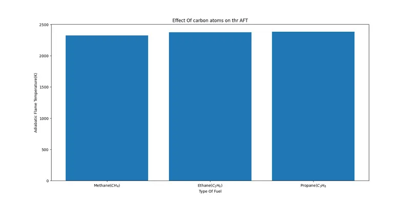
Discussion :
With more No of carbon atoms, it will produce more heat. Fuel with 3 carbon atoms produces slightly higher AFT values.
Conclusions:
Python programming for computing AFT of basic methane-air mixture reaction is computed and compared with Cantera and Effect of heat loss is studied, variation of a carbon atom and different fuel type is studied effectively.