Week 6 - Multivariate Newton Rhapson Solver

`f'(x_i) = frac(f(x_i) - f(x_(i-1)))(Deltax)`

where

`Delta x` is the step size

Given equations :

`frac(dy_1)(dt) = -0.04y_1 + 10^4 (y_2y_3)`

`frac(dy_2)(dt) = 0.04y_1 - 10^4[y_2.y_3] -3. [10^7] y_2^2`

`frac(dy_3)(dt) = 3. [10^7] . [y_2^2]`

Initial Conditions

`y_1= 1 ;y_2 = 0 ;y_3= 0`

Methods for numerical analysis

1. Implicit eluer method

2. Jacabian Method

The Newton-Raphson method (also known as Newton's method) is a technique for quickly calculating the root of a real-valued function f(x) = O. It is based on the premise that a tangent to a continuous and differentiable function might approach it. It is a method that is used to locate the roots in an iterative manner. To identify the roots, the multivariate newton's raphson approach was utilized to solve stiff systems of coupled equations. Because this is a stiff system, we'll employ the implicit differential. The multivariate Newton-Raphson technique has the following formula:

`y_1 = y_0 - [fracf(y_0)(f'(y_0))].alpha`

This process was repeated several many times

`y_(n+1) = y_n - [fracf(y_n)(f'(y_n))].alpha`

Here,

`y_(New)` is the new value that is updated after every iteration.

`y_(old)` is the old value.

`alpha` is the relaxation factor.

J is the jacobian matrix that keeps track of all possible derivates.

F is the function matrix.

Jacobian matrix is calculated numerically by finding the partial derivatives for every function with every variable and arranging it in a matrix form.

`J = [[(frac(dF_1)(dy_1))(frac(dF_1)(dy_2))(frac(dF_1)(dy_3))],[(frac(dF_2)(dy_1))(frac(dF_2)(dy_2))(frac(dF_2)(dy_3))],[(frac(dF_3)(dy_1))(frac(dF_3)(dy_2))(frac(dF_3)(dy_3))]]`

`y_(New) = y_(old) - alpha . j^-1 . F`

Derivation :

`frac(dy_1)(dt) = -0.04y_1 + 10^4 (y_2y_3)`

`frac(dy_2)(dt) = 0.04y_1 - 10^4[y_2.y_3] -3. [10^7] y_2^2`

`frac(dy_3)(dt) = 3. [10^7] . [y_2^2]`

In this challenge, initial conditions are assumed as I(for y1),0 (for y2 and y3), and simulation is done for ten minutes.

Applying initial conditions

`y_1 = 1`

`y_2 = 0`

`y_3=0`

All the equations are discretized using the backward differencing and simplifying the equations we get as

`y_1^n = y_1^(n-1) + h.(-0.04.y_1^n + 10^4.y_2^n . y_3^n)`

`y_2^n = y_2^(n-1) + h.(0.04.y_1^n - 10^4.y_2^n.y_3^n - 3.10^7.(y_2^n)^2)`

`y_3^n = y_3^(n-1) + h.(3 . 10^7(y_2^n)^2)`

Where,

h=dt

Code:

• The three given functions are defined. Then the jacobian matrix is defined.
• Here, we solve the jacobian matrix by numerical method. The general equation of the numerical differentiation is given by

`f'(x_i) = frac(f(x_i) - f(x_(i-1)))(Deltax)`

• The simulation time is taken for 10 minutes and the step size is considered 0.5
• The general structure of the code is given by
  • Outer time integration loop
  • Assembling the ODE system
  • Run newton rhapson till convergence
  • Obtain new values and update them
  • End the loop

import numpy as np 
from numpy.linalg import inv
import matplotlib.pyplot as plt

def f1(y1_old,y1,y2,y3,dt):
	return y1_old + dt*(-0.04*y1 + y2*y3*pow(10,4)) - y1

def f2(y2_old,y1,y2,y3,dt):
	return y2_old + dt*(0.04*y1 - pow(10,4)*y2*y3 - 3*pow(10,7)*pow(y2,2)) - y2 

def f3(y3_old,y1,y2,y3,dt):
	return y3_old + dt*(3*pow(10,7)*pow(y2,2)) - y3 


def jacobian(y1_old,y2_old,y3_old,y1,y2,y3,dt) :
	J = np.ones((3,3))
	h= 1e-8

	J[0,0] = (f1(y1_old,y1+h,y2,y3,dt)- f1(y1_old,y1,y2,y3,dt))/h
	J[0,1] = (f1(y1_old,y1,y2+h,y3,dt) - f1(y1_old,y1,y2,y3,dt))/h
	J[0,2] = (f1(y1_old,y1,y2,y3+h,dt) - f1(y1_old,y1,y2,y3,dt))/h

	J[1,0] = (f2(y2_old,y1+h,y2,y3,dt)- f2(y1_old,y1,y2,y3,dt))/h
	J[1,1] = (f2(y2_old,y1,y2+h,y3,dt) - f2(y1_old,y1,y2,y3,dt))/h
	J[1,2] = (f2(y2_old,y1,y2,y3+h,dt) - f2(y1_old,y1,y2,y3,dt))/h

	J[2,0] = (f3(y3_old,y1+h,y2,y3,dt)- f3(y1_old,y1,y2,y3,dt))/h
	J[2,1] = (f3(y3_old,y1,y2+h,y3,dt) - f3(y1_old,y1,y2,y3,dt))/h
	J[2,2] = (f3(y3_old,y1,y2,y3+h,dt) - f3(y1_old,y1,y2,y3,dt))/h

	return J 

dt = 1 
y1 = 1
y2 = 0
y3 = 0

y_new = np.ones((3,1))
y_old = np.ones((3,1))
y_guess = np.ones((3,1))

t = np.arange(0,600,dt)
total_iterations = len(t)
y = np.ones((3,total_iterations))

F = np.copy(y_guess)

time_iterations = 0
iterations = 0
print(y)
print(total_iterations)

for i in range(0,total_iterations):

	y_old[0] = y1
	y_old[1] = y2
	y_old[2] = y3 

	y_guess[0] = y1 
	y_guess[1] = y2 
	y_guess[2] = y3

	alpha =1 
	tolerance = 1e-8
	error = 9e9 

	while error>tolerance :
		F[0] = f1(y_old[0],y_guess[0],y_guess[1],y_guess[2],dt)
		F[1] = f2(y_old[1],y_guess[0],y_guess[1],y_guess[2],dt)
		F[2] = f3(y_old[2],y_guess[0],y_guess[1],y_guess[2],dt)

		J = jacobian(y_old[0],y_old[1],y_old[2],y_guess[0],y_guess[1],y_guess[2],dt)

		y_new = y_guess-alpha*np.matmul(inv(J),F)
		error = np.max(np.abs(y_guess-y_new))

		y_guess = y_new
		log_Message = 'iterations # = {0} y1 = {1} y2 = {2} y3 = {3}'.format(iterations,y_new[0],y_new[1],y_new[2])
		print(log_Message)
		iterations = iterations+10

	y1 = y_new[0]
	y2 = y_new[1]
	y3 = y_new[2]

	y[0,time_iterations] = y_new[0]
	y[1,time_iterations] = y_new[1]
	y[2,time_iterations] = y_new[2]

	time_iterations = time_iterations + 1 

plt.plot(t,y[0])
plt.plot(t,y[1])
plt.plot(t,y[2])
plt.xlabel('Time (sec)')
plt.ylabel('y')
plt.title('Multivariate Newton Rhapson solver dt dt = ' + str(dt))
plt.legend(['Y1','Y2','Y3'])
plt.show()

Results :

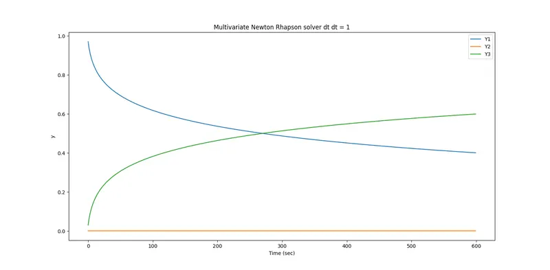
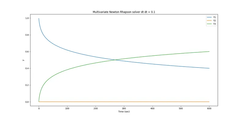
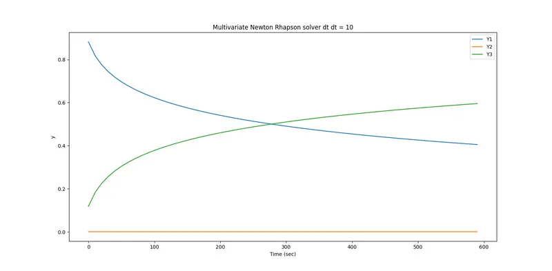
Discussion :

About the code:

Result Explanation:

We must assume the optimal value for the time step dt that produces a sufficiently accurate outcome for the issue. If we set dt to 1, the system has 600 steps, therefore the results are crisp and not very precise. However, even if the solution result is smooth, if we choose a smaller dt, such as le-2, we will have too many iterations to finish in an already complicated multivariate solver. As a result, in this example, an average dt value of 0.1 is considered to provide an accurate representation of data while also being suitably time efficient.

The results reveal that when the time step size is increased, the fluctuations in values and their domains get smaller. As a result, the appropriate time step in this scenario is 0.1