Week 3 - Pitot tube

Objecive:

1. To use Ansys to simulate the pitot tube and to conduct literature research on pitot-static tubes. Establish a link between total (stagnation) and static pressure as well.
2. Calculate the total and static pressures, as well as the velocity inaccuracy in percentages.

Introduction

Pitot tubes are used to measure fluid flow in industries to determine the velocity of a boat on the water, the velocity of an aircraft, and the velocity of gases. Pitot tubes are used to calculate the velocity of a fluid or body by measuring the pressure. Pitot tubes do not directly calculate velocity.

Pitot tubes are classified into three categories.

1. Pitot tube: A simple pitot tube is a device that measures the overall pressure of the entering fluid.
2. Static tube: Measures the entering fluid's static pressure.
3. Pitot static tube: A Pitot-static tube is being used to measure the flow velocity of liquid along a pipe.

• Measures both the total and static pressures. It'll be employed in low-speed planes. In low Mach circumstances, the measurement will be precise.
• The pitot-static tube is constructed differently from the other two tubes. It is the result of combining the characteristics of the other two tubes.
• It features a central aperture that runs the length of the tube. •It likewise has two holes on the sides and passes through the tube without making touch with the other opening to measure the overall pressure of the entering fluid. This is used to determine the entering air's static pressure.

1Q : Relationship between Total (stagnation) pressure and static pressure

The relationship between static and dynamic pressure The fluid's total pressure and velocity are as follows:

`v = root2(2((P_T -P_s)/(rho))`

Where,

v = Velocity

`P_T` = Total Pressure

`P_s` = Static Preessure

`rho` = Density

Advantages

1. They're quite small and don't have any moving components.
2. Device and installation expenses are lower.
3. It does not result in significant pressure loss.
4. Simple to integrate into the system.
5. There is no need for a separate static pressure measurement instrument, resulting in fewer mistakes.

Disadvantages :

1. Foreign particles in a fluid can block the pitot tube readily, causing abnormal readings.
2. It is less precise. Only in a specific Mach range can it perform successfully.

Why Pitot Tube is needed :

The pitot-static tube is required because airplanes rely on a variety of devices to identify their location, speed, altitude, and orientation. These systems might be very complicated, such as GPS, or very basic, such as a Pitot tube. Once the plane is in the air, it can't estimate its speed based on the rotation of the engine or the rotation of its wheels. As a result, pressure and temperature measurements are required to determine the plane's speed in mid-flight. The real speed of the airplane may be computed using the total and static pressures obtained from the pitot-static and the temperature to derive the density of the entering air.

If the flight is at a low subsonic speed, the velocity may be determined using the Relation between pressures and velocity, but at greater speeds, the calculation is more complicated and must account for compressibility effects.

Procedure :

1. Open the fluent setup and import the mesh model.
2. Input the intake velocity and pressure into the inlet boundary, and feed the same pressure into the outlet boundary since the pressure drop owing to the pitot tube is relatively small.
3. In the Viscous model, the laminar option is selected.
4. For the pitot tube, a central plane XY is formed, and the requisite outlines are projected onto it.
5. Define the appropriate static and total pressure reports in the static and total pressure tubes, respectively, as well as the required contours.
6. Using the relationship between the static, total pressure, and velocity, the velocity is computed.
7. Determine the percentage difference between the analytical and real velocity.

Setup :

Models used in simulation

Solver - Pressure based

Velocity Formulation - Absolute

Time - Steady

Viscous - Laminar flow

Boundary conditions

Inlet - Velocity inlet

Outlet - Pressure outlet

Enclosure wall - Symmetry

Static pitot tube- Wall (No slip condition)

No. of Iteration - 1000

Solution methods:

Explicit formulation is done.

Pressure based velocity coupling,

Scheme: Coupled

Spatial discretization:

gradient = Least square based

Pressure = Second order

Momentum = Second order upwind

Hybrid initialization is performed

Contours of velocity and static pressure are created at a plane created along the xy plane.

The cases are run for 1000 iterations

Results :

Case 1 :

Velocity : 240

Pressure : -2818

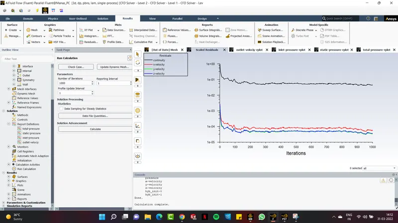
Residual Plot

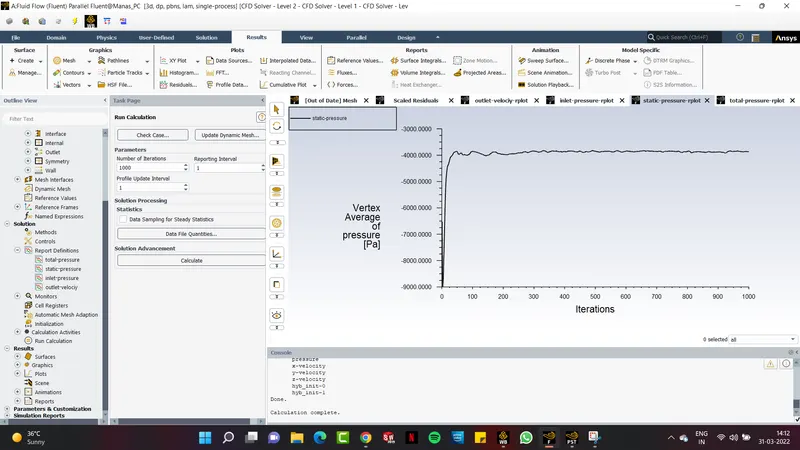
Static Pressure Plot

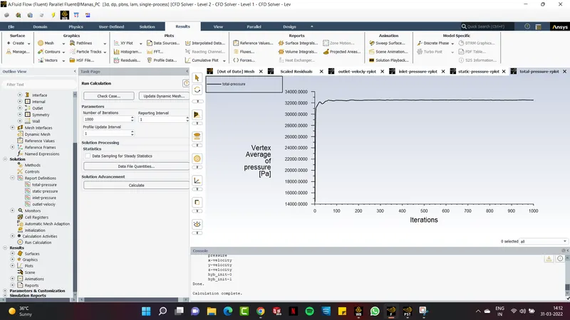
Total Pressure Plot

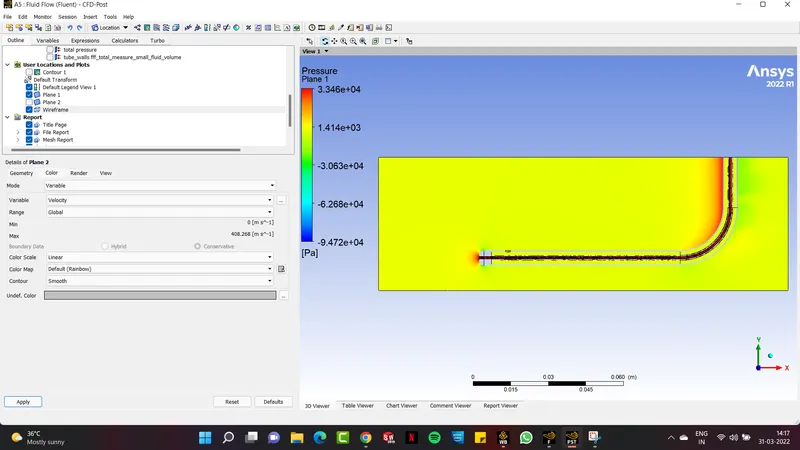
Pressure Contour

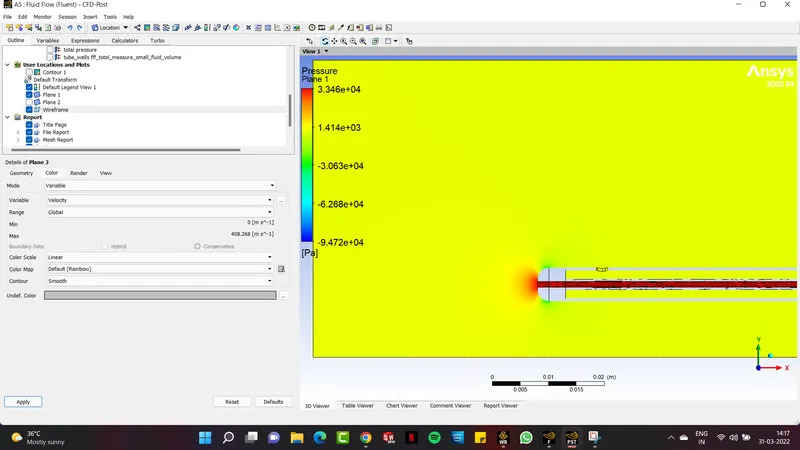
Pressure Contour

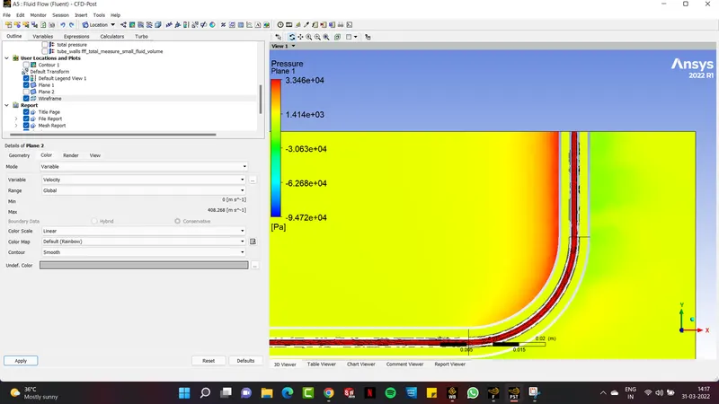
Pressure Contour

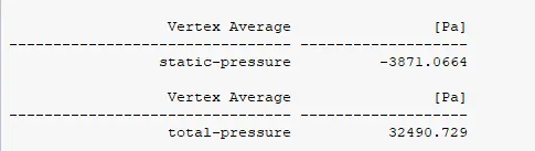
Simulated Static & Total Pressure Values

Discussion :

Total Pressure = 32490.729

Static Pressure = -3871.0664

`v = root2(2((P_T -P_s)/(rho))`

`v = root2(2((32490.729 - (-3871.0664))/1.225)`

`v = 243.65179`

Case 2 :

Velocity : 100

Pressure : 33287

Ansys Results :

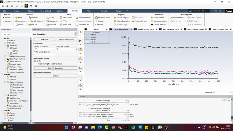
Residual Plot

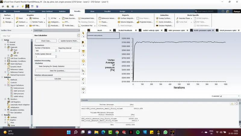
Static Pressure Plot

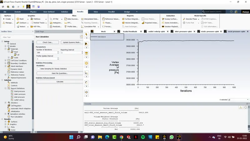
Total Pressure Plot

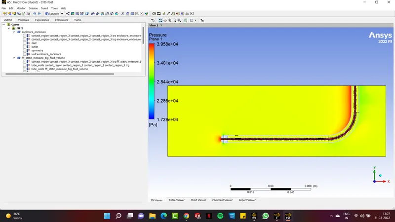
Pressure Contour

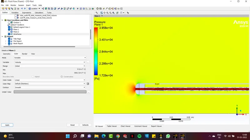
Pressure Contour

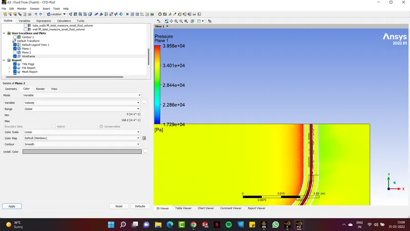
Pressure Contour

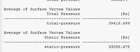
Simulated Static & Total Pressure Values

Discussion :

Total Pressure = 39418.699

Static Pressure = 33098.678

`v = root2(2((P_T -P_s)/(rho))`

`v = root2(2((39418.699 - (33098.678))/1.225)`

`v = 101.579`

Case 3 :

Velocity : 62

Pressure : 65780

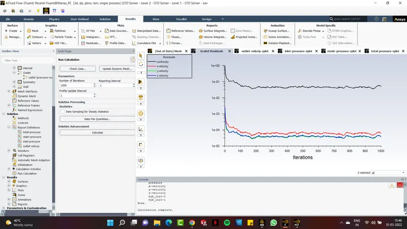
Residual Plot

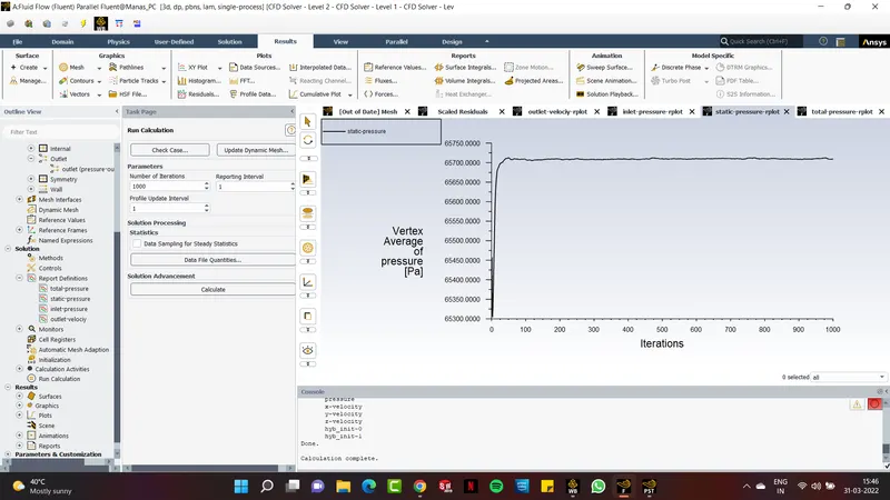
Static Pressure Plot

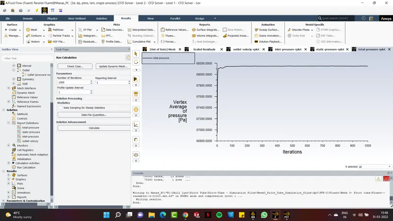
Total Pressure Plot

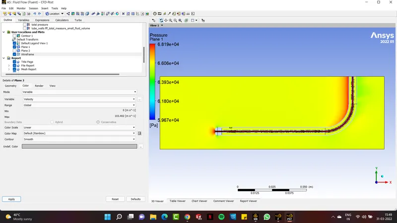
Pressure Contour

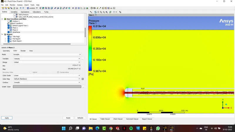
Pressure Contour

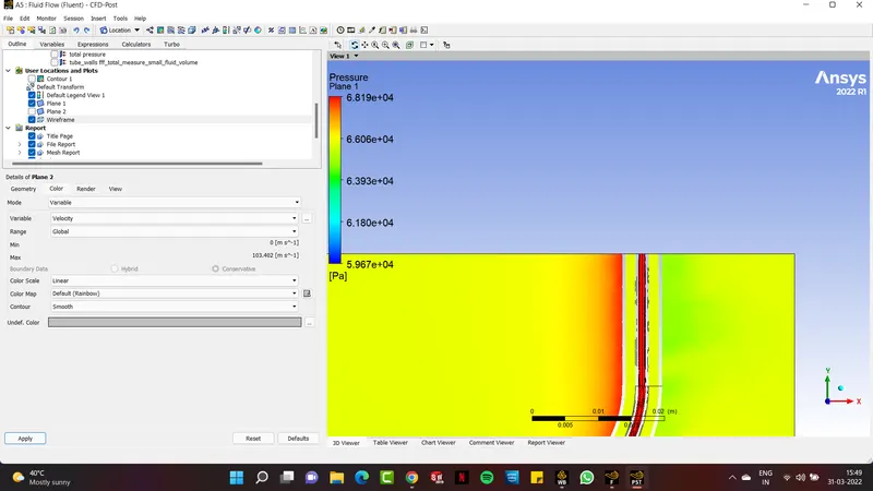
Pressure Contour

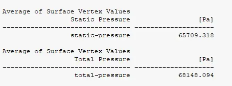
Simulated Static & Total Pressure Values

Discussion :

Total Pressure = 68148.094

Static Pressure = 65709.318

`v = root2(2((P_T -P_s)/(rho))`

`v = root2(2 ((68148.094 - (65709.318))/1.225)`

`v = 63.100`

Conclusion :

Velocity (m/s)	Pressure (pa)	Simulated - Total Pressure (pa)	Simulated - Static Pressure (pa)	Actual Velocity (m/s)	Percentage Error
240	-2818	32490.729	-3871.0664	243.65179	1.521
100	33287	39418.699	33098.678	101.579	1.579
62	65780	68148.094	65709.318	63.100	1.77

Therefore The error is calculated by comparing the real and analytical velocity values, and the error is roughly 5%, which is acceptable for this type of simulation.