Week 5 - Turbulence modelling challenge

Objectives of the problem :

1. In this challenge, you are required to do a literature review of various turbulence models explained in the Turbulence modeling video (Week-5) and explain why DNS isn’t feasible according to Kolmogorov's scale.
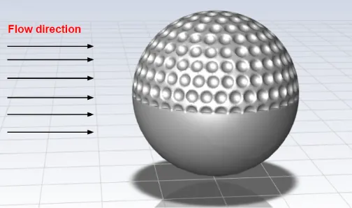
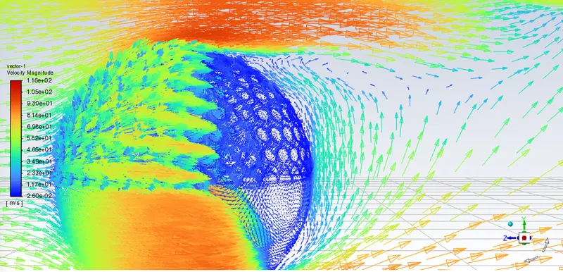
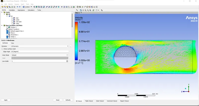
2. The below geometry performs a 3D simulation and explains the recirculation region using velocity vectors.
3. Considering the flow direction of air, the ball is traveling opposite to it at 60m/s. Explain in which direction the ball will curve by visualizing the wake region.

Solution :

Objective 1: In this challenge, you are required to do a literature review of various turbulence models explained in the Turbulence modeling video (Week-5) and explain why DNS isn’t feasible according to Kolmogorov's scale.

Part 1 :

The kind of flow is mostly determined by the Reynolds number.

Laminar flow: When the Reynolds number is smaller than the critical number, laminar flow occurs. The critical number changes depending on the geometries. The dominating forces are vicious.

Turbulent flow: Turbulent flow occurs when the Reynolds number exceeds the critical value (eddy, vortex formation begins). The forces of inertia are the most powerful.

Transition flow: The inertial and viscous forces are prominent as the flow transitions from laminar to turbulent.

In nature, laminar flows are regular, extremely stable, and predictable, whereas turbulent fluxes are very chaotic and unpredictable. Scientists averaged the disturbances into coherent structures called vortices to represent turbulent flows. These aid in the more accurate simulation of turbulent flows. There are several turbulent models available, including:

These models are classed in a variety of ways, one of which is based on the model's order.

First Order Models: Because the PDEs used to solve the turbulence in these models are of the first order, they are referred to as first-order models. This presupposes that laminar and turbulent flows are analogous. In comparison to second-order models, the average turbulent flow field is comparable to equivalent laminar flow. These models are best suited for satisfactory results with less processing power and less expense. These are commonly employed to tackle problems with turbulent viscosity.

Zero Equation model: The zero equation model does not employ PDEs to account for turbulent viscosity. The turbulent behavior of the turbulent viscosity will not be taken into consideration. The mixing length model is used to solve the turbulent viscosity directly. Eddy viscosity terms are assumed to be dimensionally equivalent to two Kolmogorov scales: length scales and velocity scales.

One equation model ( Spalart Allmaras model): A model with only one equation ( Spalart Allmaras model) The Spalart-Allmaras model is a one-equation model for kinematic eddy turbulent viscosity that solves a modeled transport equation. The Spalart-Allmaras model was created with wall-bounded flows (Internal flows) in mind, especially when the flow is linked to the body. When the mesh resolution isn't fine enough, the Spalart-Allmaras model is used to generate wall functions.

Two widely used equation Models :

1. Turbulent kinetic energy and Turbulence dissipation rate
2. Turbulent kinetic energy and Specific dissipation rate are solved using two PDEs in these models.

In the industries, the two-equation model is the most often utilized.

• K - Epsilon model: The K-epsilon model is good for turbulent flows with no flow separation. The RANS model includes this model (Reynolds averaged Navier stokes equation)

1. Standard k-epsilon: Because of its speed, this is the most extensively used model for industrial applications. To model near the wall, it employs wall functions. These models are more convergent and use less memory on the computer. The associated turbulent flows over external bodies and complicated structures produced excellent results. The downside is that it produces poor outcomes when it comes to dividing flows.
2. Realizable k-epsilon model: The modified epsilon equation model is a realizable k-epsilon model. It also shows higher performance for flows including rotation, boundary layers under significant unfavorable pressure gradients, separation, and recirculation when compared to turbulent models. In almost every comparison, Realizable k-€ outperforms the competition in terms of capturing the mean flow of complicated structures.
3. Renormalized group(RNG) k-epsilon: It features a much-enhanced epsilon equation that includes whirling effect modeling. It finds a modified version of Prandtl Number using empirical relations.

• K-omega model: The K-omega model is one of the most widely utilized in the business. The RANS model includes this model (Reynolds averaged Navier stokes equation)

1. Standard k-omega model: The standard model is a low model that may be employed for low Reynolds number flows with a relatively thick boundary layer and a viscous sublayer that can be resolved. As a result, for near-wall treatment, the conventional model is optimal. Improved performance for complicated boundary layer flows under unfavorable pressure gradients and separations is another benefit.
2. SST k-omega model: Shear stress transfer k-omega model (SST k-omega model). It's a better variant of the traditional k-omega model. It's the most common model for modeling near the wall and away from the wall, and it's the most popular model for modeling near the wall and away from the wall. Transitions from a standard model to a high Reynolds model away from the wall using a mixing technique.

Second-Order Models:

Solves transport equations for Reynolds stress terms using second-order models. These models are the most precise and are most sensitive to boundary conditions. They're also time-consuming to compute.

• Algebraic Stress Model: The algebraic Reynolds stress model is derived from the Reynolds stress dynamic equations.
• Reynolds Stress model: In inflows with high degrees of anisotropy, considerable streamline curvature, flow separation, zones of recirculating flow, or flows impacted by rotational forces, the Reynolds Stress model RM provides superior accuracy than k-omega and k epsilon.
• Turbulence on the Kolmogorov scale: Advanced theoretical fluid dynamics may be used to determine the smallest sizes of turbulence. Turbulent kinetic energy is transferred from bigger eddies to smaller eddies in the cascade process.

According to universal equilibrium theory, smaller eddies should absorb energy from bigger eddies and disperse it in about equal amounts as heat and acoustic radiation. Small scale motion is mostly determined by which bigger eddies provide energy, and

kinematic viscosity is equal to `= (dK)/(dT)`

`eta = (frac(v^3)(epsilon))^(frac(1)(4)`

`tau = (frac(v)(epsilon))^frac(1)(2)`

`v = (v.epsilon)^(1/4)`

The smallest length scale is represented by the first equation. The time scale is represented by the second equation, while the velocity scale is represented by the third equation. The most simple example is the Fourier decomposition of energy into wavenumbers.

Why, according to Kolmogorov's scale, DNS isn't viable.

• When a fluid is in a turbulent flow regime, i.e. when the flow around the body surpasses critical velocity, bigger eddies break into smaller eddies, and sometimes smaller eddies combine to form larger eddies. Energy cascading is the term for this process.
• We can't utilize DNS since it creates a very small mesh and tries to capture all anomalies (cells), therefore as the number of mesh cells grows, the time it takes to solve grows. As a result, industries dislike this strategy.

The mean flow provides energy to larger eddies.

Large eddies provide energy to smaller eddies.

• Kolmogorov's theory outlines how energy is transmitted from bigger to smaller eddies, how much energy is held by eddies of a given size, and how much energy is released by eddies of each size.
• Kolmogorov's length scale is the smallest, followed by his time scale and velocity scale

`eta = (frac(v^3)(epsilon))^(1/4)`

`eta = frac(U^3)(L)`

Where `eta` is the rate of dissipation of turbulent etic viscosity

So., the Kolmogorov time scale is given by

`t_n = (frac(v)(epsilon))^(1/2)`

to check the feasibility of the DNS

The ratio of the largest to the smallest eddies is given by

`L/eta = (L/v^(3/4))epsilon^(1/4)`

`L/eta = (L/v^(3/4))xx(U^(3/4)/L^(1/4))`

`L/eta = (LxxU^(3/4)/v)`

Therefore

`L/eta = Re^(3/4)`

• They are separated into cells holding grids to mimic the vortex, which is simple for the huge vortex. A small vortex cannot be resolved with the same grid size; thus, the grid size must be reduced for a smaller vortex.
• The issue is always to simulate the smaller vortex because as the grid size is lowered, the number of grids increases, increasing computing expenses.
• This results in a high number of 3D components, which necessitates additional computer power and time. As a result, DNS is usually avoided, however, it is nevertheless used in 2D simulations for specific scientific purposes. Given the intricacies of the architecture and the number of domains present, using DNS in industrial applications is impractical.

To comprehend Golf Ball Dynamics, we must first comprehend the lift and drag forces.

• When a body moves through the air, it experiences drag and lift forces. The drag force opposes the body's relative motion, whereas the lift force is a total upward push on the body.
• Pressure drag is caused by a pressure differential between the front and back of the body. Friction drag is caused by friction between the front and back of the body. The surface friction causes the friction drag (due to no slip near the surface there will be boundary layer formation with a gradient of velocity).
• In bluff bodies like spheres, pressure drag is considerable, but friction drag is more prominent in streamlined forms.
• In the past, golf balls were produced with smooth surfaces and did not travel as far as they do now, thus greater streamlining increases friction drag. They discovered that old golf balls go larger distances than new golf balls. It didn't take long to figure out that it was caused by the rough surface that had been formed.
• Following this discovery, golf balls were produced with flaws that were subsequently turned into dimples.
• The flow separation for a smooth ball occurs after 80 degrees in laminar flow and after 120 degrees in a turbulent flow. The pressure drag will be reduced the later the flow separation occurs. By making dimples on the ball's surface, we may make the flow turbulent.
• Turbulent flow causes more mixing or energy exchange in the boundary layer, which aids in the flow's attachment and delays flow separation.
• Once the dynamics of the cricket ball were in the big picture due to the impossible inward swing, it was discovered that air moves slowly over the rough side of the ball (high pressure) and quickly over the shiny side (low pressure), resulting in an air pressure difference that causes the net force to push the ball towards the rough side.

Simulation Steps :

• Import the geometry model and build the enclosure
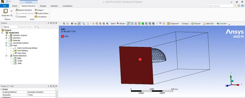
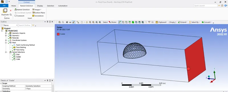
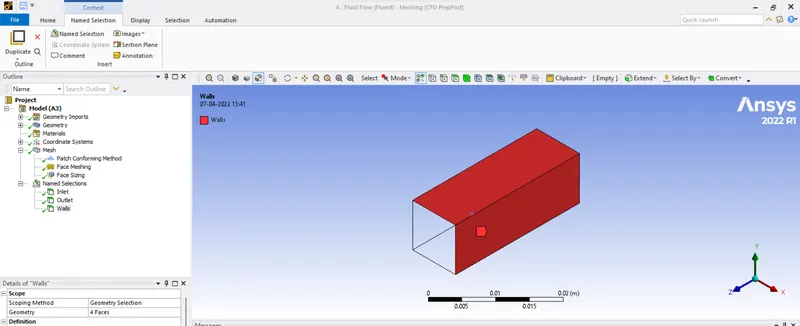
• Meshing with the right sizing and element size is accomplished. Inlets, outlets, and walls are used to name them.
• After that, the boundary conditions are entered and the kW SST solver is chosen. For both near and far from the wall, this model produces superior results.
• Proper planes and charts for pressure and velocity are constructed to display the findings.

Procedure :

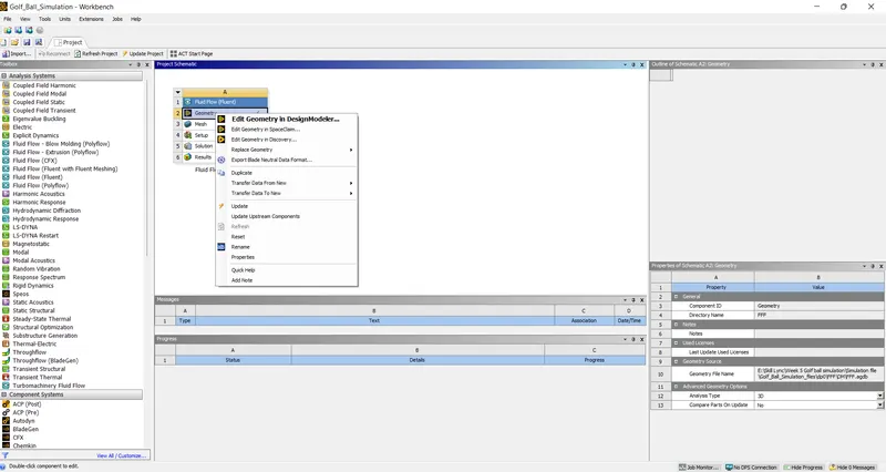
Download the geometry from the drive link and import the file to the Ansys fluent

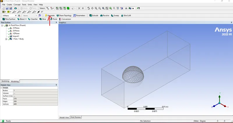
After opening your geometry in design modeler click on generate option so that your geometry will be generated

Meshing :

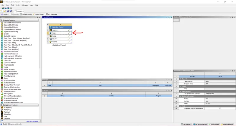
Click on edit mesh option

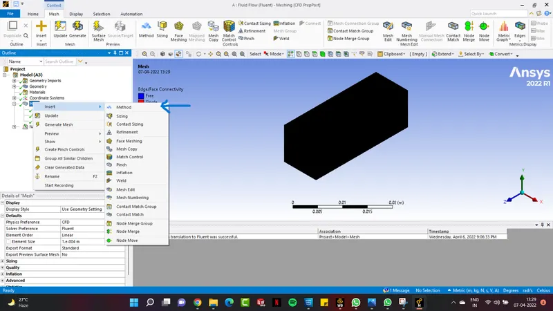
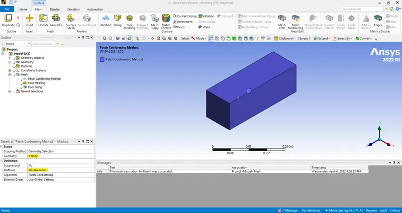
In Geometry select the body and select Tetraherons for method

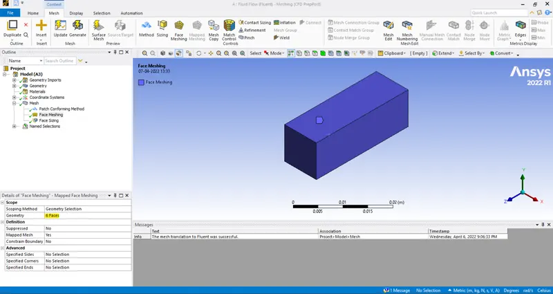
Select Face meshing and select all e 6 faces

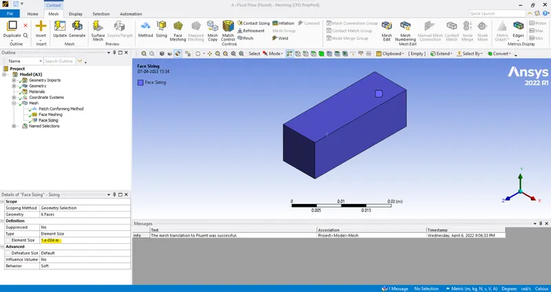
Select face sizing and give element size as 0.0001 (If the system does not support that low values of the element size we can increase the values of the element size

In mesh give the element size as 0.0001 and target skewness as 0.5 so that we can get desired mesh quality

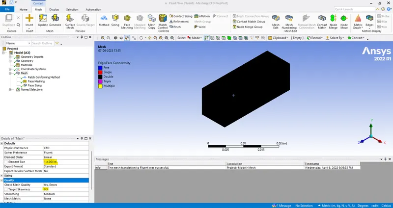
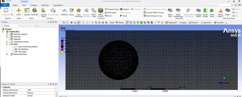
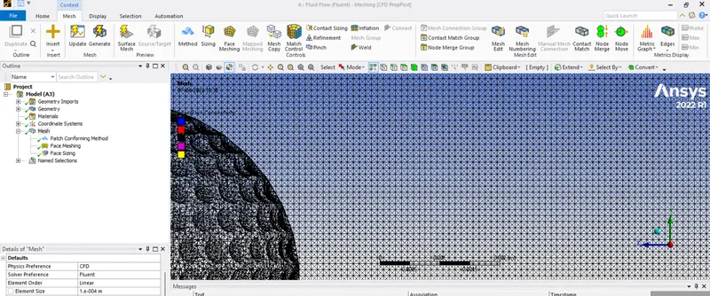
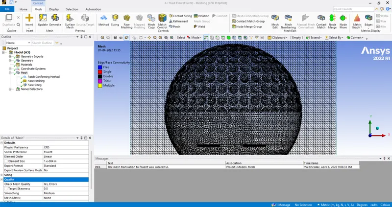
Then click on generate mesh, The final mesh looks like the blow mange

Named Section :

Name the geometry in the different sections as inlet, outlet, and walls.

Inlet :

Outlet :

Walls :

Close the mesh and open the setup

Setup the physics :

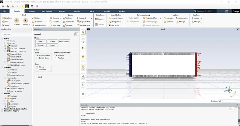
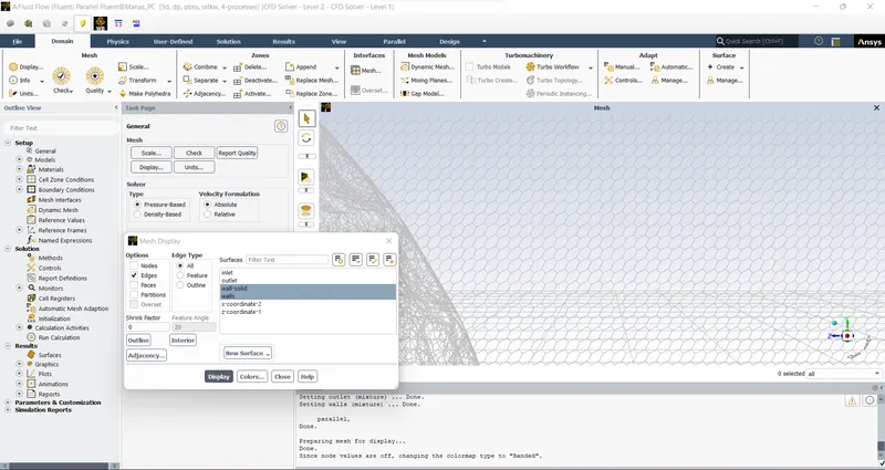
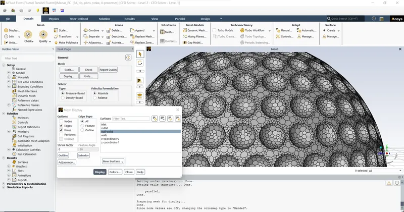
Click on display so that we can view the mesh and other sections of the geometry

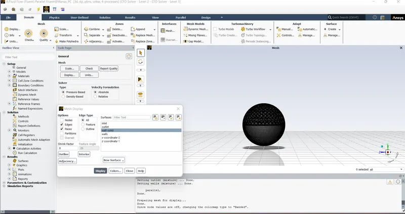
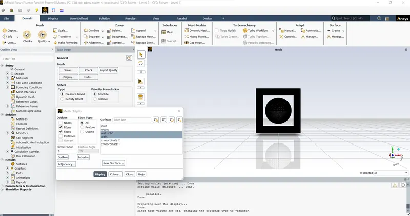
Optional Step: We can convert the tetrahedron mesh to polyhedron mesh by using the make polyhedra option. we can proceed with the existing mesh also

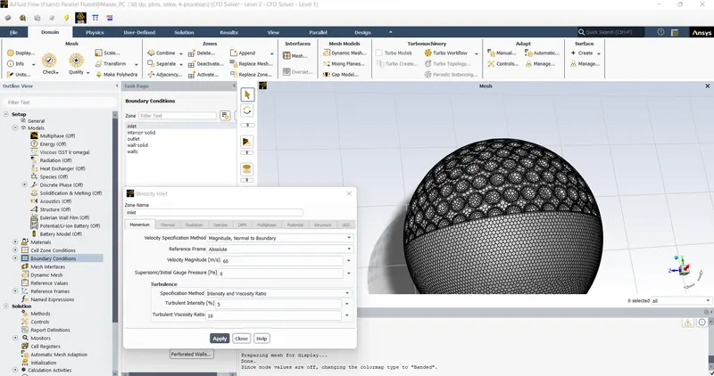
The model used: k-omega SST

The material used : air

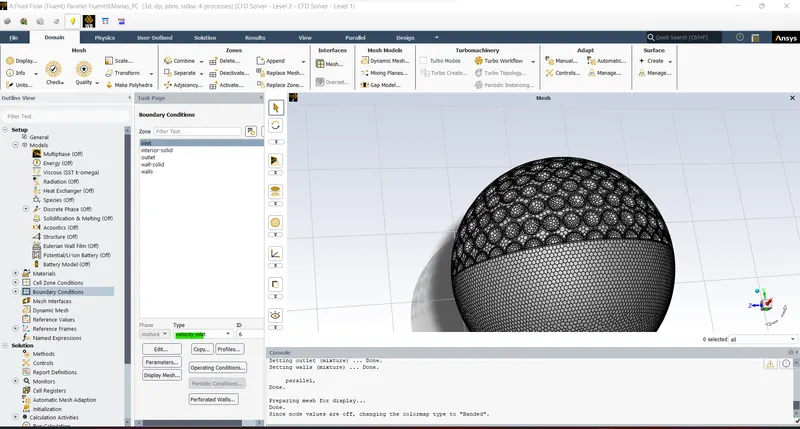
Boundary condition : Inlet - velocity inlet = v = 60m/s

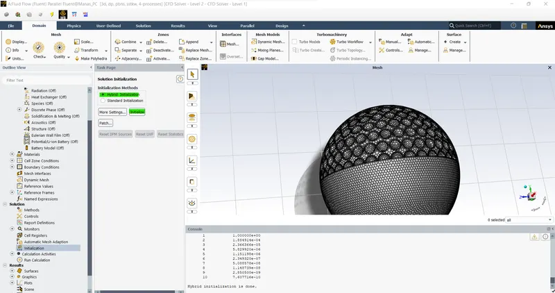
Initialize the solution :

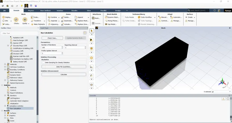
Check for case

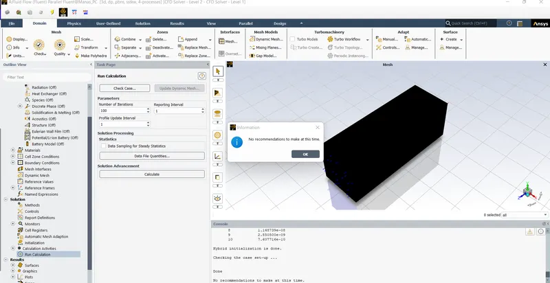
Click on calculate

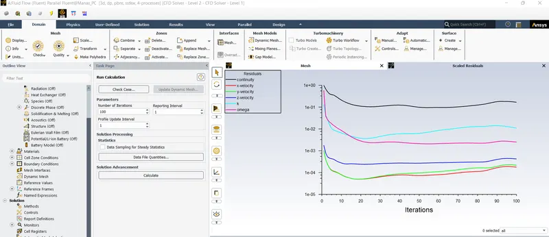
The solution is converging

Results :

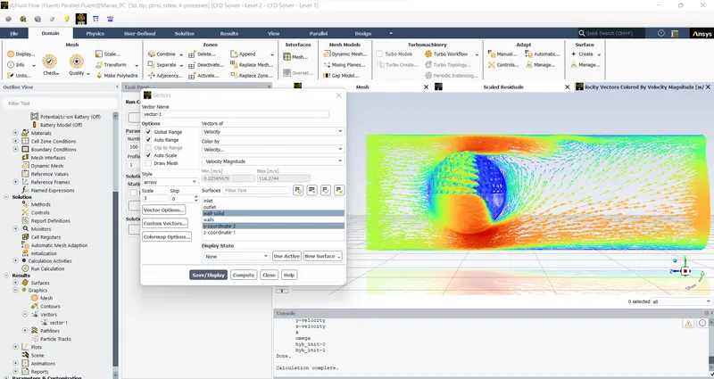
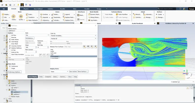
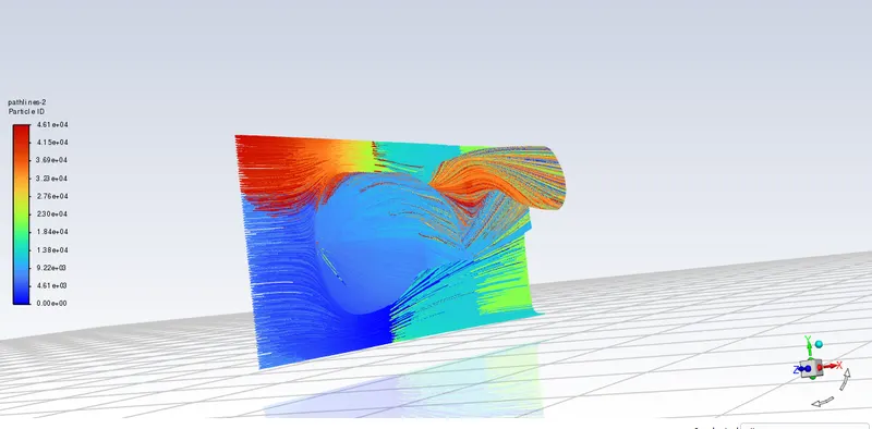
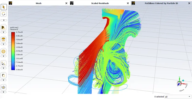
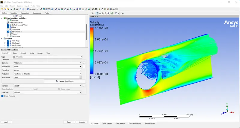
Pathlines :

Conclusion :

• We can identify the direction of the ball by looking at the velocity vectors and claim it's moving down.
• The golf ball's dimples serve to minimize drag by minimizing the wake region (recirculation).
• It also aids in the attachment of the flow and attempts to detach the flow from the golf ball.

Therefore The velocity of the flow beneath the golf ball is high, resulting in low pressure and the formation of a wake following the rough surface. The air velocity on the rough surface is lower, whereas the air velocity on the smooth surface is higher. This causes a pressure differential, which accounts for the ball's downward swing.