Week 3.5 - Deriving 4th order approximation of a 2nd order derivative using Taylor Table method

DERIVING 4th ORDER APPROXIMATION OF A 2nd ORDER DERIVATION USING TYLOR TABLE

We may encounter a partial derivative equation with a 2nd order derivative when solving a CFD problem. Because of the equation's intricacy, we may have to use a numerical technique rather than an analytical one. When using a numerical technique, however, we attempt to keep the error margin as small as feasible. We acquire more precision as the order of approximation increases.

Computing difficult grid problems require discretization as one of the most important steps. So in this challenge, we'll be dealing with how to derive 4th order approximation with the Taylors table method. We will move towards the solving of a function `exp(x)cos(x)` using the derived equation subsequently (x). The error difference of left-skewed, right-skewed, and central 4th order approximation would be compared by using both analytical and approximation.

First, let us see how we can derive the 4th order approximation for central, right-skewed, and left-skewed approximation before moving on with the programming.
Left skewed is a theory in which we only consider points on the left side of a specific grid point.
Right skewed is a theory in which we only consider points on the right side of a grid point.
The central difference method is the process by which we take data and points from both sides of the grid point, positive and negative.
Why do we need three types of 4th order approximation now, is a possible question. The answer is easy to find. Everything has to do with which approximation produces the least error.

On the other hand, while solving an equation on the boundary, we will only have points on one side, either left or right. So these are the primary reasons why we explore the many types of approximation: To reduce the chances of error and improve the stability of our results.

SOLVING MATRIESES Ax=B USING MATLAB

Before Going for Derivation of 4th order approximation solving matrices is an important step, while solving the unknown equations from the tylor table we will left out with some unknown variables or coefficients and equations containing these coefficients. in order to solve these equations we will convert them into Ax=B form

where,

A =matrix is a constant value multiplying with the unknown coefficients

B= RHS values of the equation

x = unknown variables

Matrix x is Solved by

x = `A^-1B`

Matlab Code Sovling x matrix :

clear all 
close all 
clc 

%Ax =B
%m,n are the rows and coloumsn of matrix A
%p,q are the rowns and columns of matrix B
m=input('Enter Number of Rows in matrix A: ')
n=input('Enter Number of columns in matrix A: ')
p=input('Enter Number of Rowns in matrix B: ')
q=input('Enter Number of columns matrix B: ')
for i=1:m
    for j=1:n
        a(i,j)= input('enter the elements of the matrix A ')
    end
end
a=reshape(a,m,n)
for k=1:p
    for j=1:q
        b(k,j) = input('enter the elements of the matrix B ')
    end
end
x=inv(a)*b

By using the above code we can find The matrix x

Derivation of 4th order approximation of the second-order derivative :

Central difference method:

The numerical stencil of the central difference method is given by

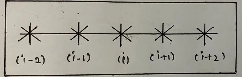
We're computing the 4th order approximation at point (i), where we're going to take information from the four points around i.e., two points to the left of i and two points to the right of i. Let's call those sites (i-2), (i-1), (i+1), and (i+2), respectively, and the distance between them is (`Deltax`). As seen in the illustration above, our number stencil will appear like this.

The hypothesis equation for the above stencil is given by

`frac(del^2u)(delx^2)` = a`f(i-2)`+b`f(i-1)`+c`f(i)`+d`f(i+1)`+e`f(i+2)`

To find the coefficients (a,b,c,d,e) of the above equation tylor method is used

`af(i-2)` = `af_(i)`-`frac(af'_i(2Deltax))(1!)`+`frac(af''_i(2Deltax)^2)(2!)`-`frac(af'''_i(2Deltax)^3)(3!)`+`frac(af''''_i(2Deltax)^4)(4!)`-`frac(af'''''_i(2Deltax)^5)(5!)`+`frac(af''''''_i(2Deltax)^6)(6!)`+......

`bf_(i-1)` = `bf_(i)`-`frac(bf'_i(Deltax))(1!)`+`frac(bf''_i(Deltax)^2)(2!)`-`frac(bf'''_i(Deltax)^3)(3!)`+`frac(bf''''_i(Deltax)^4)(4!)`-`frac(bf'''''_i(Deltax)^5)(5!)`+`frac(bf''''''_i(Deltax)^6)(6!)`+.....`

`cf_i` = `cf_i`

`df_(i+1)` = `df_(i)`+`frac(df'_i(Deltax))(1!)`+`frac(df''_i(Deltax)^2)(2!)`+`frac(df'''_i(Deltax)^3)(3!)`+`frac(df''''_i(Deltax)^4)(4!)`+`frac(df'''''_i(Deltax)^5)(5!)`+`frac(df''''''_i(Deltax)^6)(6!)`+.....`

`ef_(i+2)` = `ef_(i)`+`frac(ef'_i(2Deltax))(1!)`+`frac(ef''_i(2Deltax)^2)(2!)`+`frac(ef'''_i(2Deltax)^3)(3!)`+`frac(ef''''_i(2Deltax)^4)(4!)`+`frac(ef'''''_i(2Deltax)^5)(5!)`+`frac(ef''''''_i(2Deltax)^6)(6!)`+......

By arranging the above tylor series and converting them into tylor table we get :

	`f(i)`	`Deltaxf'(i)`	`Deltax^2f''(i)`	`Deltax^3f'''(i)`	`Deltax^4f''''(i)`	`Deltax^5f'''''(i)`	`Deltax^6f''''''(i)`
`af(i-2)`	a	-2a	`frac(4a)(2)`	`-frac(8a)(6)`	`frac(16a)(24)`	`-frac(32a)(120)`	`frac(64a)(240)`
`bf_(i-1)`	b	-b	`frac(b)(2)`	`-frac(b)(6)`	`frac(b)(24)`	`-frac(b)(120)`	`frac(b)(240)`
`cf_i`	c	0	0	0	0	0	0
`df_(i+1)`	d	d	`frac(d)(2)`	`frac(d)(6)`	`frac(d)(24)`	`frac(d)(120)`	`frac(d)(240)`
`ef_(i+2)`	e	2e	`frac(4e)(2)`	`frac(8e)(6)`	`frac(16e)(24)`	`frac(32e)(120)`	`frac(64e)(240)`
`sum(af_(i-2)+bf_(i-1)+cf_(i)+df_(i+1)+ef_(i+2))`	0	0	1	0	0	?	?

We have five unknow variables and five equations with the unknowns by sovling these 5 equations we get the coefficients (a,b,c,d,e)

`a+b+c+d+e=0`

`-2a-b+0+d+2e=0`

`frac(4a)(2)+frac(b)(2)+0+frac(d)(2)+frac(4e)(2)=1`

`-frac(8a)(6)-frac(b)(6)+0+ frac(d)(6)+ frac(8e)(6)=0`

`frac(16a)(24)+frac(b)(24)+0+frac(d)(24)+frac(16e)(24) =0`

Coverting the above equations into matrix form we get :

`[[1,1,1,1,1],[-2,-1,0,1,2],[2,1/2,0,1/2,2],[-8/6,-1/6,0,1/6,8/6],[16/24,1/24,0,1/24,16/24]]` `[(a),(b),(c),(d),(e)]` = `[(0),(0),(1),(0),(0),(0)]`

The above matrix is in the form Ax=b

A = `[[1,1,1,1,1],[-2,-1,0,1,2],[2,1/2,0,1/2,2],[-8/6,-1/6,0,1/6,8/6],[16/24,1/24,0,1/24,16/24]]`

B = `[(0),(0),(1),(0),(0)]`

x = `[(a),(b),(c),(d),(e)]`

to find the x matrix = `A^-1B`

By using the matlab code for solving x matrix we get

x = `[(a),(b),(c),(d),(e)]` = `[(-0.0833),(1.3333),(-2.5000),(1.3333),(-0.0833)]`

Skewed right-sided difference :

The numerical stencil of the Skewed right-sided difference method is given by

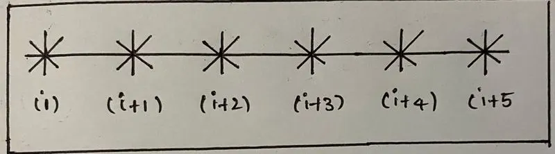
We're computing the 4th order approximation at point (i), where we're going to take information from the next five points around. Let's call those sites (i+1), (i+2), (i+3), (i+4) and (i+5) respectively, and the distance between them is (`Deltax`). As seen in the illustration above, our number stencil will appear like this.

The hypothesis equation for the above stencil is given by

`frac(del^2u)(delx^2)` = `af_(i)+bf_(i+1)+cf_(i+2)+df_(i+3)+ef_(i+4)+gf_(i+5)`

To find the coefficients (a,b,c,d,e,g) of the above equation Tylor method is used

`af_i` = `af_i`

`bf_(i+1)` = `bf_(i)`+`frac(bf'_i(Deltax))(1!)`+`frac(bf''_i(Deltax)^2)(2!)`+`frac(bf'''_i(Deltax)^3)(3!)`+`frac(bf''''_i(Deltax)^4)(4!)`+`frac(bf'''''_i(Deltax)^5)(5!)`+`frac(bf''''''_i(Deltax)^6)(6!)`+.....`

`cf_(i+2)` = `cf_(i)`+`frac(cf'_i(2Deltax))(1!)`+`frac(cf''_i(2Deltax)^2)(2!)`+`frac(cf'''_i(2Deltax)^3)(3!)`+`frac(cf''''_i(2Deltax)^4)(4!)`+`frac(cf'''''_i(2Deltax)^5)(5!)`+`frac(cf''''''_i(2Deltax)^6)(6!)`+......

`df_(i+3)` = `df_(i)`+`frac(df'_i(3Deltax))(1!)`+`frac(df''_i(3Deltax)^2)(2!)`+`frac(df'''_i(3Deltax)^3)(3!)`+`frac(df''''_i(3Deltax)^4)(4!)`+`frac(df'''''_i(3Deltax)^5)(5!)`+`frac(df''''''_i(3Deltax)^6)(6!)`+......

`ef_(i+4)` = `ef_(i)`+`frac(ef'_i(4Deltax))(1!)`+`frac(ef''_i(4Deltax)^2)(2!)`+`frac(ef'''_i(4Deltax)^3)(3!)`+`frac(ef''''_i(4Deltax)^4)(4!)`+`frac(ef'''''_i(4Deltax)^5)(5!)`+`frac(ef''''''_i(4Deltax)^6)(6!)`+......

`gf_(i+5)` = `gf_(i)`+`frac(gf'_i(5Deltax))(1!)`+`frac(gf''_i(5Deltax)^2)(2!)`+`frac(gf'''_i(5Deltax)^3)(3!)`+`frac(gf''''_i(5Deltax)^4)(4!)`+`frac(gf'''''_i(5Deltax)^5)(5!)`+`frac(gf''''''_i(5Deltax)^6)(6!)`+......

By arranging the above tylor series and converting them into tylor table we get :

	`f(i)`	`Deltaxf'(i)`	`Deltax^2f''(i)`	`Deltax^3f'''(i)`	`Deltax^4f''''(i)`	`Deltax^5f'''''(i)`	`Deltax^6f''''''(i)`
`af_i`	a	0	0	0	0	0	0
`bf_(i+1)`	b	b	`frac(b)(2)`	`frac(b)(6)`	`frac(b)(24)`	`frac(b)(120)`	`frac(b)(720)`
`cf_(i+2)`	c	2c	`frac(4c)(2)`	`frac(8c)(6)`	`frac(16c)(24)`	`frac(32c)(120)`	`frac(64c)(720)`
`df_(i+3)`	d	3d	`frac(9d)(2)`	`frac(27d)(6)`	`frac(81d)(24)`	`frac(243d)(120)`	`frac(729d)(720)`
`ef_(i+4)`	e	4e	`frac(16e)(2)`	`frac(64e)(6)`	`frac(256e)(24)`	`frac(1024e)(120)`	`frac(4096e)(720)`
`gf_(i+5)`	g	5g	`frac(25g)(2)`	`frac(125g)(6)`	`frac(625g)(24)`	`frac(3125g)(120)`	`frac(15625g)(720)`
`sum(af_(i)+bf_(i+1)+cf_(i+2)+df_(i+3)+ef_(i+4)+gf_(i+5))`	0	0	1	0	0	0	?

We have six unknow variables and five equations with the unknowns by sovling these 6 equations we get the coefficients (a,b,c,d,e,g)

`a+b+c+d+e+g=0`

`0+b+2c+3d+4e+5g=0`

`0+frac(b)(2)+frac(4c)(2)+ frac(9d)(2)+frac(16e)(2)+frac(25g)(2) =1`

`0+frac(b)(6)+ frac(8c)(6)+frac(27d)(6)+frac(64e)(6)+frac(125g)(6) =0`

`0+frac(b)(24)+frac(16c)(24)+frac(81d)(24)+frac(256e)(24)+frac(625g)(24)=0`

`0+frac(b)(120)+frac(32c)(120)+frac(243d)(120)+frac(1024e)(120)+frac(3125g)(120)=0`

Coverting the above equations into matrix form we get :

`[[1,1,1,1,1,1],[0,1,2,3,4,5],[0,1/2,2,9/2,8,25/2],[0,1/6,8/6,27/6,64/6,125/6],[0,1/24,16/24,81/24,256/24,625/24],[0,1/120,32/120,243/120,1024/120,3125/120]]` `[(a),(b),(c),(d),(e),(g)]` = `[(0),(0),(1),(0),(0),(0)]`

The above matrix is in the form Ax=b

A = `[[1,1,1,1,1,1],[0,1,2,3,4,5],[0,1/2,2,9/2,8,25/2],[0,1/6,8/6,27/6,64/6,125/6],[0,1/24,16/24,81/24,256/24,625/24],[0,1/120,32/120,243/120,1024/120,3125/120]]`

B = `[(0),(0),(1),(0),(0),(0)]`

x = `[(a),(b),(c),(d),(e),(g)]`

to find the x matrix = `A^-1B`

By using the matlab code for solving x matrix we get

x = `[(a),(b),(c),(d),(e),(g)]` = `[(3.7500),(-12.8333),(17.8333),(-13.0000),(5.0833),(-0.8333)]`

Skewed left-sided difference:

The numerical stencil of the Skewed left-sided difference method is given by

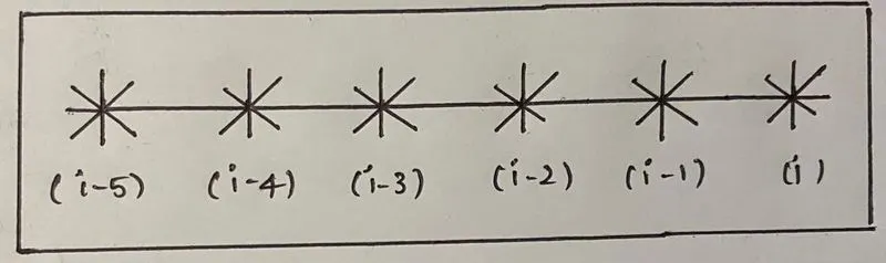
We're computing the 4th order approximation at point (i), where we're going to take information from the previous five points around. Let's call those sites (i-1), (i-2), (i-3), (i-4) and (i-5) respectively, and the distance between them is (`Deltax`). As seen in the illustration above, our number stencil will appear like this.

The hypothesis equation for the above stencil is given by

`frac(del^2u)(delx^2)` = `af_(i-5)+bf_(i-4)+cf_(i-3)+df_(i-2)+ef_(i-1)+gf_i`

To find the coefficients (a,b,c,d,e,g) of the above equation tylor method is used

`af(i-5)` = `af_(i)`-`frac(af'_i(5Deltax))(1!)`+`frac(af''_i(5Deltax)^2)(2!)`-`frac(af'''_i(5Deltax)^3)(3!)`+`frac(af''''_i(5Deltax)^4)(4!)`-`frac(af'''''_i(5Deltax)^5)(5!)`+`frac(af''''''_i(5Deltax)^6)(6!)`+......

`bf(i-4)` = `bf_(i)`-`frac(bf'_i(4Deltax))(1!)`+`frac(bf''_i(4Deltax)^2)(2!)`-`frac(bf'''_i(4Deltax)^3)(3!)`+`frac(bf''''_i(4Deltax)^4)(4!)`-`frac(bf'''''_i(4Deltax)^5)(5!)`+`frac(bf''''''_i(4Deltax)^6)(6!)`+......

`cf(i-3)` = `cf_(i)`-`frac(cf'_i(3Deltax))(1!)`+`frac(cf''_i(3Deltax)^2)(2!)`-`frac(cf'''_i(3Deltax)^3)(3!)`+`frac(cf''''_i(3Deltax)^4)(4!)`-`frac(cf'''''_i(3Deltax)^5)(5!)`+`frac(cf''''''_i(3Deltax)^6)(6!)`+......

`df(i-2)` = `df_(i)`-`frac(af'_i(2Deltax))(1!)`+`frac(df''_i(2Deltax)^2)(2!)`-`frac(df'''_i(2Deltax)^3)(3!)`+`frac(df''''_i(2Deltax)^4)(4!)`-`frac(df'''''_i(2Deltax)^5)(5!)`+`frac(df''''''_i(2Deltax)^6)(6!)`+......

`ef_(i-1)` = `ef_(i)`-`frac(ef'_i(Deltax))(1!)`+`frac(ef''_i(Deltax)^2)(2!)`-`frac(ef'''_i(Deltax)^3)(3!)`+`frac(ef''''_i(Deltax)^4)(4!)`-`frac(ef'''''_i(Deltax)^5)(5!)`+`frac(ef''''''_i(Deltax)^6)(6!)`+.....`

`gf_i` = `gf_i`

By arranging the above tylor series and converting them into tylor table we get :

	`f(i)`	`Deltaxf'(i)`	`Deltax^2f''(i)`	`Deltax^3f'''(i)`	`Deltax^4f''''(i)`	`Deltax^5f'''''(i)`	`Deltax^6f''''''(i)`
`af(i-5)`	a	`-5a`	`frac(25a)(2)`	`-frac(125a)(6)`	`frac(625a)(24)`	`-frac(3125a)(120)`	`frac(15625a)(720)`
`bf(i-4)`	b	`-4b`	`8b`	`-frac(64b)(6)`	`frac(256b)(24)`	`-frac(1024b)(120)`	`frac(4096b)(720)`
`cf(i-3)`	c	`-3c`	`frac(9c)(2)`	`-frac(27c)(6)`	`frac(81c)(24)`	`-frac(243c)(120)`	`frac(729c)(120)`
`df(i-2)`	d	`-2d`	`2d`	`-frac(8d)(6)`	`frac(16d)(24)`	`-frac(32d)(120)`	`frac(64d)(720)`
`ef_(i-1)`	e	`-e`	`frac(e)(2)`	`-frac(e)(6)`	`frac(e)(24)`	`-frac(e)(120)`	`frac(e)(720)`
`gf_i`	g	0	0	0	0	0	0
`sum(af_(i-5)+bf_(i-4)+cf_(i-3)+df_(i-2)+ef_(i-1)+gf_i)`	0	0	1	0	0	0	?

We have six unknow variables and five equations with the unknowns by sovling these 6 equations we get the coefficients (a,b,c,d,e,g)

`a+b+c+d+e+g=0`

`-5a-4b-3c-2d-e+0=0`

`frac(25a)(2)+8b+frac(9c)(2)+2d+frac(e)(2)+0 =1`

`-frac(125a)(6)-frac(64b)(6)-frac(27c)(6)-frac(8d)(6)-frac(e)(6)+0=0`

`frac(625a)(24)+frac(256b)(24)+frac(81c)(24)+frac(16d)(24)+frac(e)(24)+0=0`

`-frac(3125a)(120)-frac(1024b)(120)-frac(243c)(120)-frac(32d)(120)-frac(e)(120)+0=0`

Coverting the above equations into matrix form we get :

`[[1,1,1,1,1,1],[-5,-4,-3,-2,-1,0],[25/2,16/2,9/2,4/2,1/2,0],[-125/6,-64/6,-27/6,-8/6,-1/6,0],[625/24,256/24,81/24,2/3,1/24,0],[-3125/120,-128/15,-81/40,-4/15,-1/120,0]]` `[(a),(b),(c),(d),(e),(g)]` = `[(0),(0),(1),(0),(0),(0)]`

The above matrix is in the form Ax=b

A = `[[1,1,1,1,1,1],[-5,-4,-3,-2,-1,0],[25/2,16/2,9/2,4/2,1/2,0],[-125/6,-64/6,-27/6,-8/6,-1/6,0],[625/24,256/24,81/24,2/3,1/24,0],[-3125/120,-128/15,-81/40,-4/15,-1/120,0]]`

B = `[(0),(0),(1),(0),(0),(0)]`

x = `[(a),(b),(c),(d),(e),(g)]`

to find the x matrix = `A^-1B`

By using the matlab code for solving x matrix we get

x = `[(a),(b),(c),(d),(e),(g)]` = `[ (-0.8333),(5.0833),(-13.0000),(17.8333),(-12.8333),(3.7500)]`

Matlab Program to derive second-order derivative of the given function exp(x)*cos(x) and compare it with the numerical approximation

First Write the program for Solving Matrix Ax=B, because to find the coefficients of the hypothesis equations of the central difference method, Skewed right Side difference method and Skewed Left side difference method

function [X] = Matrixmultiplication(m,n,p,q)
%Ax =B
%m,n are the rows and coloumsn of matrix A
%p,q are the rowns and columns of matrix B
%m=input('Enter Number of Rows in matrix A: ')
%n=input('Enter Number of columns in matrix A: ')
%p=input('Enter Number of Rowns in matrix B: ')
%q=input('Enter Number of columns matrix B: ')
for i=1:m
    for j=1:n
        a(i,j)= input('enter the elements of the matrix A ')
    end
end
a=reshape(a,m,n)
for k=1:p
    for j=1:q
        b(k,j) = input('enter the elements of the matrix B ')
    end
end
X = inv(a)*b
end

Save the file as Matrixmultiplication.m file in order to call the function in the main program

Main code: Deriving 4th order approximation of a 2nd order derivative of given function exp(x)*cos(x) using hypothesis equation and comparing it with the numerical approximation

clear all
close all
clc

%given Function = exp(x)*cos(x)
X=pi/3;
dx=linspace(pi/4,pi/4000,40);
analytical_derivative = -2*exp(X)*sin(X);


%Central difference method
disp('Enter the matrix a and b for central difference method')
x= Matrixmultiplication(5,5,5,1);
a=x(1);
b=x(2);
c=x(3);
d=x(4);
e=x(5);

for i=1:length(dx)
Central_difference_method(i) = ((a*exp(X-2*dx(i))*cos(X-2*dx(i)))+(b*exp(X-dx(i))*cos(X-dx(i)))+(c*exp(X)*cos(X))+(d*exp(X+dx(i))*cos(X+dx(i)))+(e*exp(X+2*dx(i))*cos(X+2*dx(i))))/(dx(i))^2;
end
%Skewed right-sided difference method
disp('Enter the matrix a and b for Skewed right-sided difference method')
y =Matrixmultiplication(6,6,6,1);
a=y(1);
b=y(2);
c=y(3);
d=y(4);
e=y(5);
g=y(6);

for i=1:length(dx)
Skewed_right_sided_difference_method(i) = ((a*exp(X)*cos(X))+(b*exp(X+dx(i))*cos(X+dx(i)))+(c*exp(X+2*dx(i))*cos(X+2*dx(i)))+(d*exp(X+3*dx(i))*cos(X+3*dx(i)))+(e*exp(X+4*dx(i))*cos(X+4*dx(i)))+(g*exp(X+5*dx(i))*cos(X+5*dx(i))))/(dx(i))^2;
end

%Skewed left-sided difference
disp('Enter the matrix a and b for Skewed left-sided difference')
z=Matrixmultiplication(6,6,6,1);
a=z(1);
b=z(2);
c=z(3);
d=z(4);
e=z(5);
g=z(6);

for i=1:length(dx)
Skewed_left_sided_difference(i)=((g*exp(X)*cos(X))+(e*exp(X-dx(i))*cos(X-dx(i)))+(d*exp(X-2*dx(i))*cos(X-2*dx(i)))+(c*exp(X-3*dx(i))*cos(X-3*dx(i)))+(b*exp(X-4*dx(i))*cos(X-4*dx(i)))+(a*exp(X-5*dx(i))*cos(X-5*dx(i))))/(dx(i))^2;
end

Central_difference_method(i)
Skewed_right_sided_difference_method(i)
Skewed_left_sided_difference(i)


%error calculation
for i=1:length(dx)
Central_difference_method_error(i) = abs(Central_difference_method(i)-analytical_derivative)
Skewed_right_sided_difference_method_error(i)=abs(Skewed_right_sided_difference_method(i)-analytical_derivative)
Skewed_left_sided_difference_error(i) = abs(Skewed_left_sided_difference(i)-analytical_derivative)
end

%plotting of graphs
figure(1)
plot(dx,Central_difference_method_error,'r','linewidth',2)
hold on
grid on 
plot(dx,Skewed_right_sided_difference_method_error,'g','linewidth',2)
hold on
plot(dx,Skewed_left_sided_difference_error,'b','linewidth',2)
xlabel('dx')
ylabel('Error value')
legend('Central difference method error','Skewed right sided difference method error','Skewed left sided difference error')

figure(2)
loglog(dx,Central_difference_method_error,'r','linewidth',2)
hold on
grid on 
loglog(dx,Skewed_right_sided_difference_method_error,'b','linewidth',2)
hold on
loglog(dx,Skewed_left_sided_difference_error,'g','linewidth',2)
xlabel('dx')
ylabel('Error value')
legend('Central difference method error','Skewed right sided difference method error','Skewed left sided difference error')

Results :

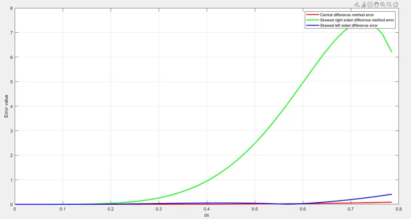
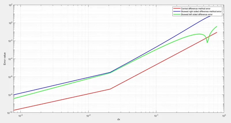
Discussion :

1. After looking at the graphs of error vs. 'dx for central, skewed right-sided, and skewed left-sided difference 4th order errors, it's clear that the central difference approximation produces more accurate solutions and thus produces fewer errors than the right-skewed and left-skewed difference schemes.

2. As can be shown, the central differencing scheme produces more perfect solutions or minimum error than the skewed difference scheme. However, using central differencing to assess solutions is not always feasible. If we wish to compute numerical approximations for a function at a boundary or corner node, we can't utilise the central difference approach since it requires data from both sides of the node or border in this case. Since a result, the skewed difference approach plays an important role in this case, as data from one side may be utilised to compute numerical approximation at a point in the skewed scheme.