Project 1- Creating your own openFOAM solver
Aim: Creating your own OpenFOAM solver, and Running a cavity test case with the created solver
Procedure: Here in this challenge we are trying to solve the scalar transport equation in the solver, we are using icoFoam solver for this challenge
The scalar transport equation is defined as:
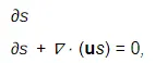
where s is the scalar quantity being transported by the velocity u.
Temperature is a scalar property we are using for this challenge
Step by step Procedure is explained below with the respective images.
Step 1: Make a Working Directory
Step 2: Parallelly go to the Openfoam Solvers folder and find the incompressible folder and then find the icoFoam solver Folder
Step 3: Copy the icoFoam solver folder to your working directory
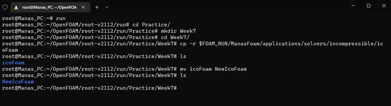
Step 4: Rename the Solver folder to your Choice (In my case NewIcoFoam)
Step 5: Go inside the solver (NewIcoFoam) folder, We can see .C file and .H file.
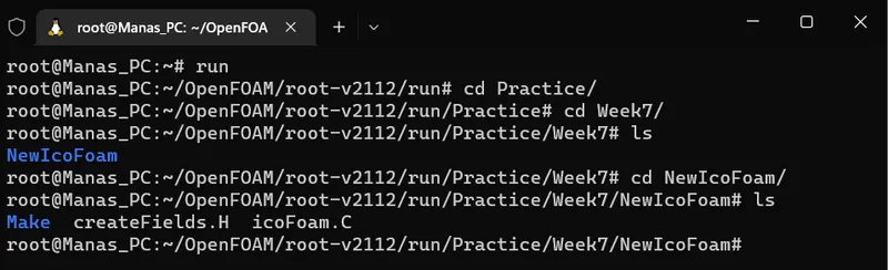
We are going to edit all the Folder and files Step by step
Step 6: First go Inside your icoFoam.C file, We can see the equations of momentum, pressure, and velocity is been solved in the code. Copy the Momentum predictor code and paste the code just after the velocity calculation loop. As shown in the figure (Line 158 - 167)
/*---------------------------------------------------------------------------*\
  =========                 |
  \\      /  F ield         | OpenFOAM: The Open Source CFD Toolbox
   \\    /   O peration     |
    \\  /    A nd           | www.openfoam.com
     \\/     M anipulation  |
-------------------------------------------------------------------------------
    Copyright (C) 2011-2016 OpenFOAM Foundation
    Copyright (C) 2019 OpenCFD Ltd.
-------------------------------------------------------------------------------
License
    This file is part of OpenFOAM.

    OpenFOAM is free software: you can redistribute it and/or modify it
    under the terms of the GNU General Public License as published by
    the Free Software Foundation, either version 3 of the License, or
    (at your option) any later version.

    OpenFOAM is distributed in the hope that it will be useful, but WITHOUT
    ANY WARRANTY; without even the implied warranty of MERCHANTABILITY or
    FITNESS FOR A PARTICULAR PURPOSE.  See the GNU General Public License
    for more details.

    You should have received a copy of the GNU General Public License
    along with OpenFOAM.  If not, see <http://www.gnu.org/licenses/>.

Application
    NewIcoFoam

Group
    grpIncompressibleSolvers

Description
    Transient solver for incompressible, laminar flow of Newtonian fluids.

    \heading Solver details
    The solver uses the PISO algorithm to solve the continuity equation:

        \f[
            \div \vec{U} = 0
        \f]

    and momentum equation:

        \f[
            \ddt{\vec{U}}
          + \div \left( \vec{U} \vec{U} \right)
          - \div \left(\nu \grad \vec{U} \right)
          = - \grad p
        \f]

    Where:
    \vartable
        \vec{U} | Velocity
        p       | Pressure
    \endvartable

    \heading Required fields
    \plaintable
        U       | Velocity [m/s]
        p       | Kinematic pressure, p/rho [m2/s2]
    \endplaintable

\*---------------------------------------------------------------------------*/

#include "fvCFD.H"
#include "pisoControl.H"

// * * * * * * * * * * * * * * * * * * * * * * * * * * * * * * * * * * * * * //

int main(int argc, char *argv[])
{
    argList::addNote
    (
        "Transient solver for incompressible, laminar flow"
        " of Newtonian fluids."
    );

    #include "postProcess.H"

    #include "addCheckCaseOptions.H"
    #include "setRootCaseLists.H"
    #include "createTime.H"
    #include "createMesh.H"

    pisoControl piso(mesh);

    #include "createFields.H"
    #include "initContinuityErrs.H"

    // * * * * * * * * * * * * * * * * * * * * * * * * * * * * * * * * * * * //

    Info<< "\nStarting time loop\n" << endl;

    while (runTime.loop())
    {
        Info<< "Time = " << runTime.timeName() << nl << endl;

        #include "CourantNo.H"

        // Momentum predictor

        fvVectorMatrix UEqn
        (
            fvm::ddt(U)
          + fvm::div(phi, U)
          - fvm::laplacian(nu, U)
        );

        if (piso.momentumPredictor())
        {
            solve(UEqn == -fvc::grad(p));
        }

        // --- PISO loop
        while (piso.correct())
        {
            volScalarField rAU(1.0/UEqn.A());
            volVectorField HbyA(constrainHbyA(rAU*UEqn.H(), U, p));
            surfaceScalarField phiHbyA
            (
                "phiHbyA",
                fvc::flux(HbyA)
              + fvc::interpolate(rAU)*fvc::ddtCorr(U, phi)
            );

            adjustPhi(phiHbyA, U, p);

            // Update the pressure BCs to ensure flux consistency
            constrainPressure(p, U, phiHbyA, rAU);

            // Non-orthogonal pressure corrector loop
            while (piso.correctNonOrthogonal())
            {
                // Pressure corrector

                fvScalarMatrix pEqn
                (
                    fvm::laplacian(rAU, p) == fvc::div(phiHbyA)
                );

                pEqn.setReference(pRefCell, pRefValue);

                pEqn.solve(mesh.solver(p.select(piso.finalInnerIter())));

                if (piso.finalNonOrthogonalIter())
                {
                    phi = phiHbyA - pEqn.flux();
                }
            }

            #include "continuityErrs.H"

            U = HbyA - rAU*fvc::grad(p);
            U.correctBoundaryConditions();

        }
        //Scalar Equation Solver
        fvScalarMatrix SEqn
        (
            fvm::ddt(S)
          + fvm::div(phi, S)       //Flux Term
          - fvm::laplacian(DS, S)  //Diffusive Term
        );

        SEqn.solve();
        S.correctBoundaryConditions();

        runTime.write();

        runTime.printExecutionTime(Info);
    }

    Info<< "End\n" << endl;

    return 0;
}


// ************************************************************************* //
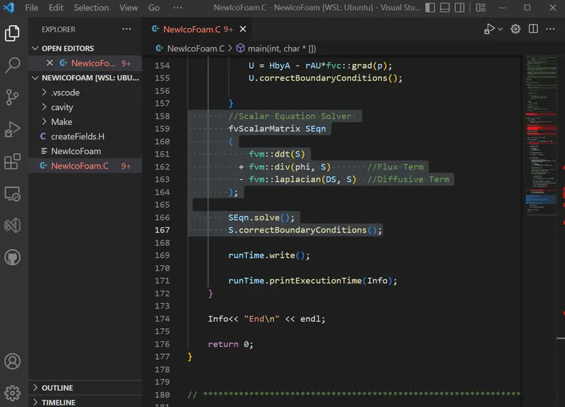
Explanation: Here we Are typing to solve a scaler quantity S, S can be any Scalar quantity. So using the Finite Volume Method scheme we are trying to solve time derivative, flux Term, and Diffusive term.
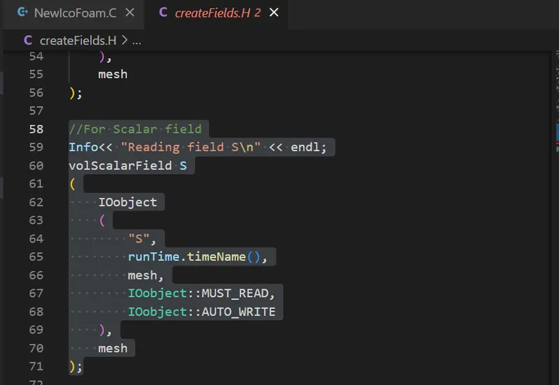
Step 7: Updating The createFields.H, adding scalar Field, and creating Scalar IOobject. adding lines from 58-71. Scalar IOobject is created
Info<< "Reading transportProperties\n" << endl;

IOdictionary transportProperties
(
    IOobject
    (
        "transportProperties",
        runTime.constant(),
        mesh,
        IOobject::MUST_READ_IF_MODIFIED,
        IOobject::NO_WRITE
    )
);

dimensionedScalar nu
(
    "nu",
    dimViscosity,
    transportProperties
);

dimensionedScalar DS
(
    "DS",
    dimViscosity,
    transportProperties
);

Info<< "Reading field p\n" << endl;
volScalarField p
(
    IOobject
    (
        "p",
        runTime.timeName(),
        mesh,
        IOobject::MUST_READ,
        IOobject::AUTO_WRITE
    ),
    mesh
);


Info<< "Reading field U\n" << endl;
volVectorField U
(
    IOobject
    (
        "U",
        runTime.timeName(),
        mesh,
        IOobject::MUST_READ,
        IOobject::AUTO_WRITE
    ),
    mesh
);

//For Scalar field
Info<< "Reading field S\n" << endl;
volScalarField S
(
    IOobject
    (
        "S",
        runTime.timeName(),
        mesh,
        IOobject::MUST_READ,
        IOobject::AUTO_WRITE
    ),
    mesh
);

#include "createPhi.H"


label pRefCell = 0;
scalar pRefValue = 0.0;
setRefCell(p, mesh.solutionDict().subDict("PISO"), pRefCell, pRefValue);
mesh.setFluxRequired(p.name());
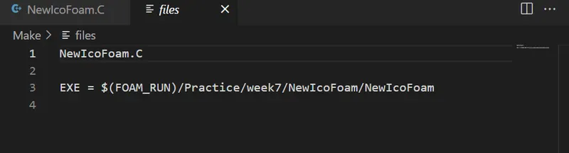
Step 8: Now we need to edit the "make" file. Edit the "files" file in the make file by changing the Name of the .C (icoFoam.C) file to NewIcoFoam.C which we saved outside the make file
Step 9: Everything is set, For making your own Solver for the test case.
Check Table
| Name of the files | Checked |
| NewIcoFoam.C | Done |
| icoFoam.H | Done |
| Make/files | Done |
Step 10: Run "wmake" command. If it is a successful run, Then the created solver along with the scalar field is compiled successfully. (In My case it's successful)
Step 11: It's the second Phase of setting the file for the solver. copy the "p" file and paste it into the same folder by changing the name of the file to S. This is to set up the dimensions and boundary condition for the scalar vector.
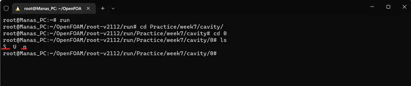
Step 12: In this case, we are considering the Temperature of the scalar quantity. so set the dimension to
/*--------------------------------*- C++ -*----------------------------------*\
| =========                 |                                                 |
| \\      /  F ield         | OpenFOAM: The Open Source CFD Toolbox           |
|  \\    /   O peration     | Version:  v2112                                 |
|   \\  /    A nd           | Website:  www.openfoam.com                      |
|    \\/     M anipulation  |                                                 |
\*---------------------------------------------------------------------------*/
FoamFile
{
    version     2.0;
    format      ascii;
    class       volScalarField;
    object      S;
}
// * * * * * * * * * * * * * * * * * * * * * * * * * * * * * * * * * * * * * //

dimensions      [0 0 0 1 0 0 0];

internalField   uniform 500;

boundaryField
{
    movingWall
    {
        type            fixedValue;
        value           uniform 550.0;
    }

    fixedWalls
    {
        type            fixedValue;
        value           uniform 500.0;
    }

    frontAndBack
    {
        type            empty;
    }
}


// ************************************************************************* //
Step 13: Once the scalar dimensions are given properly, we need to edit the transportporperties file in the constants folder. We need to add the dS coefficient in the transportporperties file so that the governing equation which we gave in the solver can be solved.
/*--------------------------------*- C++ -*----------------------------------*\
| =========                 |                                                 |
| \\      /  F ield         | OpenFOAM: The Open Source CFD Toolbox           |
|  \\    /   O peration     | Version:  v2112                                 |
|   \\  /    A nd           | Website:  www.openfoam.com                      |
|    \\/     M anipulation  |                                                 |
\*---------------------------------------------------------------------------*/
FoamFile
{
    version     2.0;
    format      ascii;
    class       dictionary;
    object      transportProperties;
}
// * * * * * * * * * * * * * * * * * * * * * * * * * * * * * * * * * * * * * //

nu              0.01;
DS              0.0025;


// ************************************************************************* //
Step 14: Once the transportproperties are set properly, we need to edit the controlDict file, By changing the application name and also the simulation time if needed. (In my case the application name will be NewIcoFoam and the simulation time will be 1.0 sec)
/*--------------------------------*- C++ -*----------------------------------*\
| =========                 |                                                 |
| \\      /  F ield         | OpenFOAM: The Open Source CFD Toolbox           |
|  \\    /   O peration     | Version:  v2112                                 |
|   \\  /    A nd           | Website:  www.openfoam.com                      |
|    \\/     M anipulation  |                                                 |
\*---------------------------------------------------------------------------*/
FoamFile
{
    version     2.0;
    format      ascii;
    class       dictionary;
    object      controlDict;
}
// * * * * * * * * * * * * * * * * * * * * * * * * * * * * * * * * * * * * * //

application     NewIcoFoam;

startFrom       startTime;

startTime       0;

stopAt          endTime;

endTime         1.0;

deltaT          0.005;

writeControl    timeStep;

writeInterval   20;

purgeWrite      0;

writeFormat     ascii;

writePrecision  6;

writeCompression off;

timeFormat      general;

timePrecision   6;

runTimeModifiable true;


// ************************************************************************* //
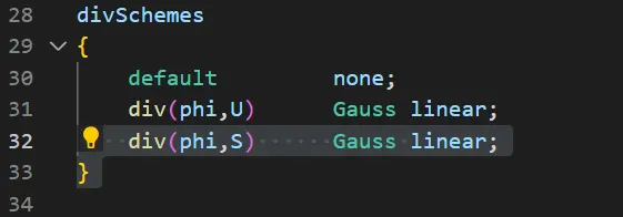
Step 15: Once all the inputs in the controldict are given properly, we should look into the fvSchemes file where we need to add the type of fvScheme that should be used to solve the scalar transport equation. (In My case I used Gauss linear scheme) to solve the Transport Equation
/*--------------------------------*- C++ -*----------------------------------*\
| =========                 |                                                 |
| \\      /  F ield         | OpenFOAM: The Open Source CFD Toolbox           |
|  \\    /   O peration     | Version:  v2112                                 |
|   \\  /    A nd           | Website:  www.openfoam.com                      |
|    \\/     M anipulation  |                                                 |
\*---------------------------------------------------------------------------*/
FoamFile
{
    version     2.0;
    format      ascii;
    class       dictionary;
    object      fvSchemes;
}
// * * * * * * * * * * * * * * * * * * * * * * * * * * * * * * * * * * * * * //

ddtSchemes
{
    default         Euler;
}

gradSchemes
{
    default         Gauss linear;
    grad(p)         Gauss linear;
}

divSchemes
{
    default         none;
    div(phi,U)      Gauss linear;
    div(phi,S)      Gauss linear;
}

laplacianSchemes
{
    default         Gauss linear orthogonal;
}

interpolationSchemes
{
    default         linear;
}

snGradSchemes
{
    default         orthogonal;
}


// ************************************************************************* //
Step 16: once the fvScheme is set properly, we need to look into fvSolutions files, in this file we need to set the solver, preconditioner, Tolerance, and reltol values so that the solution will take place with the given values.
| Parameter | Value |
| Solver |
PBiCG
|
| Preconditioner |
DILU
|
| Tolerance |
1e-09
|
| reltol |
0
|
/*--------------------------------*- C++ -*----------------------------------*\
| =========                 |                                                 |
| \\      /  F ield         | OpenFOAM: The Open Source CFD Toolbox           |
|  \\    /   O peration     | Version:  v2112                                 |
|   \\  /    A nd           | Website:  www.openfoam.com                      |
|    \\/     M anipulation  |                                                 |
\*---------------------------------------------------------------------------*/
FoamFile
{
    version     2.0;
    format      ascii;
    class       dictionary;
    object      fvSolution;
}
// * * * * * * * * * * * * * * * * * * * * * * * * * * * * * * * * * * * * * //

solvers
{
    p
    {
        solver          PCG;
        preconditioner  DIC;
        tolerance       1e-06;
        relTol          0.05;
    }

    pFinal
    {
        $p;
        relTol          0;
    }

    U
    {
        solver          smoothSolver;
        smoother        symGaussSeidel;
        tolerance       1e-05;
        relTol          0;
    }

    S
    {
        solver          PBiCG;
        preconditioner  DILU;
        tolerance       1e-09;
        relTol          0;
    }
}

PISO
{
    nCorrectors     2;
    nNonOrthogonalCorrectors 0;
    pRefCell        0;
    pRefValue       0;
}


// ************************************************************************* //
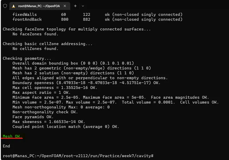
Step 17: Once all the settings are made properly, Run "BlockMesh" command, and the run the "chechMesh" command. Once the mesh is ok we can now run the executable inside the test case folder
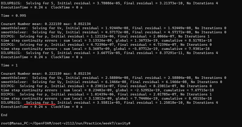
Step 18: Run the executable. In my case ./NewIcoFoam . We can see the Simulation is carried out sucessfully for 1.0 sec and the saclar quantity is been calculated at every time step.
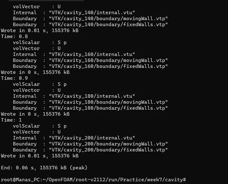
Step 19: Run "foamToVTK" Command to view the results in Paraview.
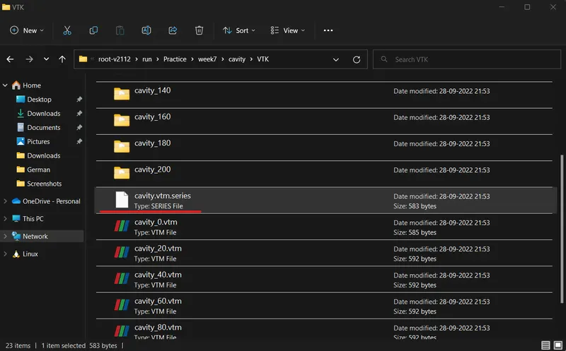
Step 20: Now run "explorer.exe ." and then open VTK Folder and then open cavity.vtk.series file in paraview

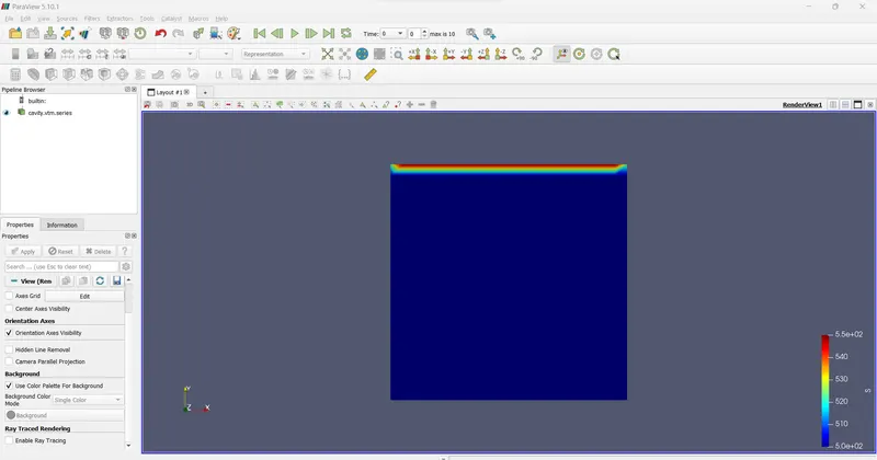
Results :
Initial Condition
Final Condition
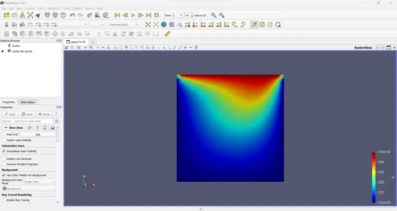
Discussion: From the above results we can see the simulation is run for 10 sec with given boundary conditions along with the given scalar transport Equation
Note: The scalar quantity we used here is Temperature
Changes in the solver:
• Replace the main working equation with:
Answer: Added the transport equation in the .C file where the main Equation is been solved
• What change will you make in the create fields.H file (Hint: the p field is originally created here)
Answer: In The createFields.H, add scalar Field, and create Scalar IOobject. We can see in the "step 7" images, adding lines from 58-71. Scalar IOobject is created
• Compile scalarFoam using wmake. How are the Make/files modified?
Answer: Edit the "files" file in the make file by changing the Name of the .C (icoFoam.C) file to NewIcoFoam.C which we saved outside the make file. It is clearly explained in Step 8
Changes in the case:
• Use the $FOAM_TUTORIALS/incompressible/icoFoam/cavity case to test out your solver. Rename it scalarCavity.
Answer : I used the same test case for the Scalar solver.
• The scalar transport equation has no pressure p to solve, instead a scalar s. What changes will you make in the 0 folders?
Answer : Copy the "p" file and paste it into the same folder by changing the name of the file to S. This is to set up the dimensions and boundary condition for the scalar vector.
In this case, we are considering the Temperature of the scalar quantity. so set the dimension to
• You will have to change the interpolation scheme in fvSchemes to account for the ∇ · (us) term. How will you do this?
Answer: we need to add the type of fvScheme that should be used to solve the scalar transport equation. (In My case I used Gauss linear scheme) to solve the Transport Equation. It is explained in step 15 clearly.
• In fvSolutions, a solver has to be specified for the quantity s. Can you just replace this with the solver used for p?
Answer: fvSolutions files, in this file we need to set the solver, preconditioner, Tolerance, and reltol values so that the solution will take place with the given values.
| Parameter | Value |
| Solver |
PBiCG
|
| Preconditioner |
DILU
|
| Tolerance |
1e-09
|
| reltol |
0
|
• Run this case by making the appropriate change in controlDict.
Answer: changing the application name and also the simulation time if needed. (In my case the application name will be NewIcoFoam and the simulation time will be 1.0 sec) in step 14 it was clearly explained
Conclusion: Hence The Cavity test case is solved by using the Scalar transport equation (In this case scalar quantity is temperature ) where the scalar quantity being transported by the velocity u.