Week 8- Moving zones approach in Fluent

Objective :

1. What are the approaches by which you would model moving zones?
2. Which approach would you use to model unsteady phenomena?
3. Simulate rotary motion for the geometry given
   1. Plot the velocity profile of the fluid motion

Solution :

In fluid flow, there are two forms of motion: rectilinear and rotating motion.

Modeling rotational motion may be done in two ways:

• Moving reference frame
• Moving mesh approach.

Moving reference frame:

A Moving Reference Frame (MRF) is a steady-state Computational Fluid Dynamics modeling approach for simulating rotating equipment that is very simple, robust, and efficient. MRFs may be used to model the rotors of a quadcopter, for example.

The main purpose of using a moving reference frame is to make a problem that is unstable in the stationary (inertial) frame stable in the moving frame. It is feasible to transfer the equations of fluid motion to the rotating frame in order to get steady-state solutions for a steadily rotating frame (i.e., the rotational speed is constant). Fluent allows the activation of a moving reference frame with a constant rotational speed by default. The modified equations will have extra terms that are not included in the fluent formulation if the rotational speed is not constant. Moving reference frames with constant rotational speed can be used to study unstable simulations. For several zones, there are two techniques. It's a steady-state approximation in which variable rotational and translational speeds can be attributed to distinct cell zones. The moving reference frame equations are used to solve the flow in each moving cell zone. The equations simplify to their stationary versions when the zone is stationary (w = 0). A local reference frame transformation is conducted at the interfaces between cell zones to allow flow variables from one zone to be utilized to compute fluxes at the border of the neighboring zone. In Section 2, we'll go through the MRF interface formulation in greater depth.

It's worth noting that the MRF method ignores the relative motion of a moving zone in relation to surrounding zones (which might be moving or stationary); the mesh stays constant during the computation. This is similar to stopping the motion of a moving element in a given position and measuring the instantaneous flow field while the rotor is in that position. As a result, the MRF is also known as the "frozen rotor strategy." While the MRF method is clearly an approximation, it can produce a suitable flow model in many situations. The MRF model, for example, can be employed in turbomachinery applications when the rotor-stator interaction is mild and the flow at the interface between the moving and stationary zones is reasonably simple. Large-scale transient effects are not present in mixing tanks, for example, since the impeller-baffle interactions are rather mild. Therefore, the MRF model may be utilized. The MRF model may also be used to calculate a flow field that can be utilized as an initial condition for a transient sliding mesh computation. The multiple reference frame model should not be utilized since it avoids the requirement for a starting computation; nevertheless, if it is important to mimic the transients that may occur in powerful rotor-stator interactions, the sliding mesh model alone should be employed.

There are two types of moving reference frame approaches:

• Single moving reference frame.
• Multiple moving reference frame that uses a mixing plane approach.

Contact region or the interface :

• This is the region existing in contact with the stationary plane or the moving plane.
• Section or region of intersection of the two frames.

Circular type of interface :

• The Navier stokes equation is the stationary frame and the moving frame is solved separately.
• Data is transferred from one frame to another through the interface

There are three methods of data transfer namely:

• Area Averaging Method
• Mixed approach

In this approach, the partial differential equations are solved. the momentum equation, energy equation, and continuity equation are solved simultaneously.

Moving mesh approach :

This approach gives the best result.

• Unsteady flows are modeled using the moving mesh method. Generally, vortex-induced flows are employed, and moving mesh approaches are used for flows including vortex contact with bodies. Physical PDEs and a mesh equation generated from the equidistribution of an error metric (referred to as the monitor function) are solved concurrently in moving mesh techniques, and meshes are dynamically concentrated on steep sections.

Simulation of the geometry:

1. The meshed model is imported into Ansys fluent.
2. A preliminary mesh check is done.
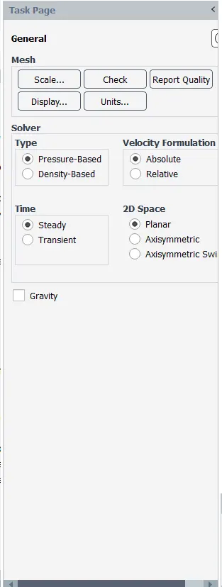
3. Under the general conditions, Pressure based solver is used. Steady-state analysis is performed. Generally, with moving reference frames, steady-state studies are conducted.. 2d planar analysis is done.
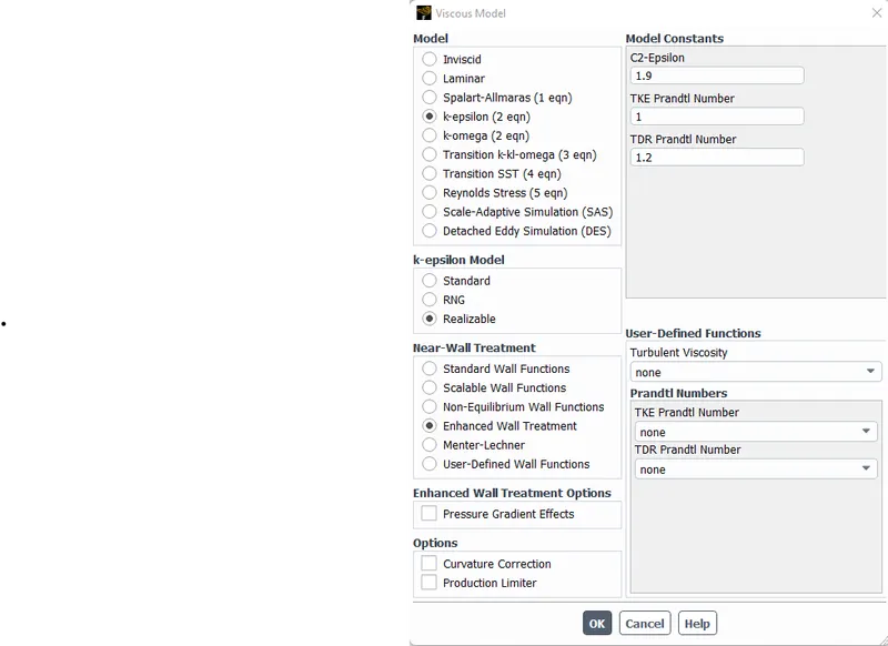
4. Under the model's tab, turbulence modeling is performed. both k omega ST and K epsilon model give satisfactory results, but in this project, RNG K -epsilon model is used for analysis.
5. The material for analysis is air.
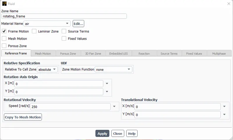
6. In the cell zones, under the zones, a rotating frame is enabled. Frame motion box is checked.

Setup :

The origin of the rotation axis is set to (0,0), which is fine for this model. ls, this model's angular velocity is 250 rpm. There are two methods to alter the angular velocity units in fluent: either the value of the angular velocity is changed to radian per second or the units of the angular velocity are changed to rpm.

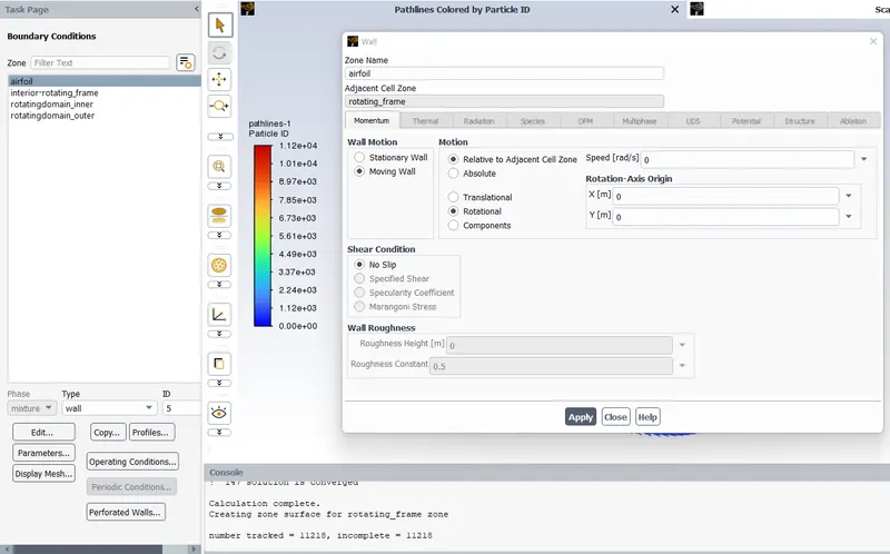
The boundary condition, Moving wall boundary condition is applied to the airfoil, Which is relative to the adjacent cell zone. The rotational motion needed to be allowed

Results :

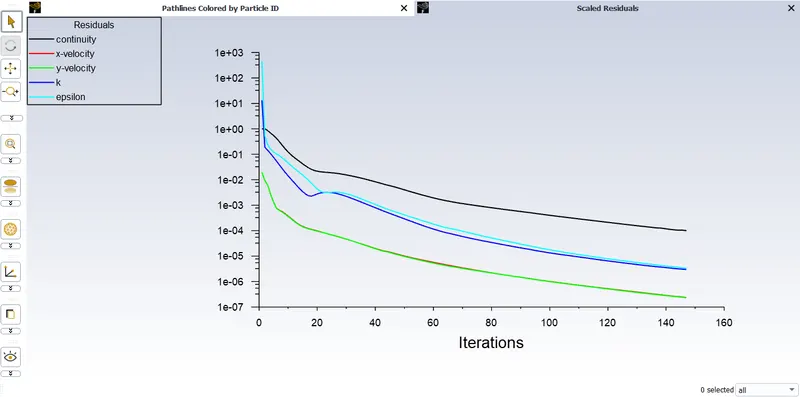
Resuduals :

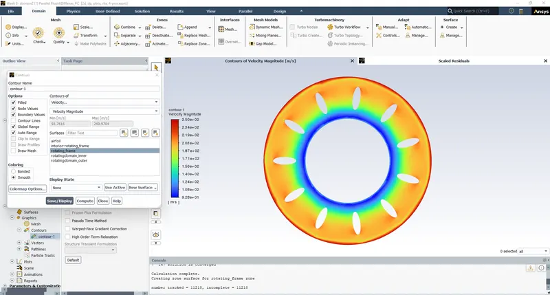
Velocity Contours

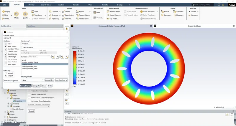
Pressure Contours :

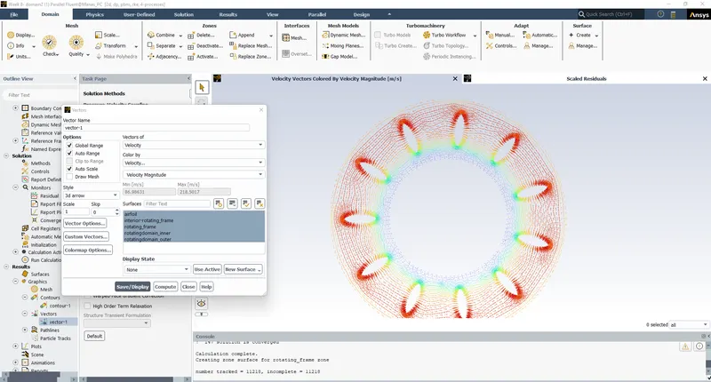
Velocity vector :

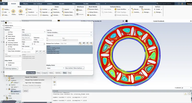
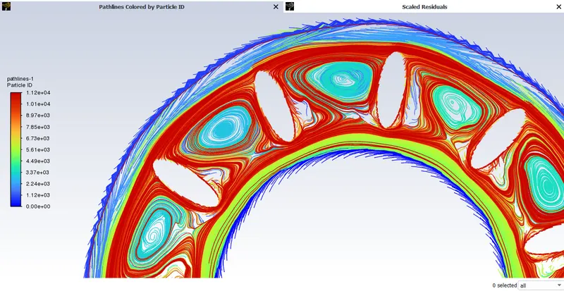
Pathlines velocity :

Conclusion :

1. The largest velocity was observed in the outside frame in velocity contour plots, whereas the lowest velocity was recorded near the inner frame. However, by observing the airfoil edges, the top edge has been exposed to the most velocity, while the lower edge has been exposed to the lowest velocity. On top of the airfoil, the velocity separation can also be seen.
2. Because the suction of air takes place near the center of the impeller, the static pressure contour plot shows a low-pressure zone there. The velocity rises as it approaches the trailing edge of the airfoil until it reaches the impeller's maximum diameter.