Week 4 - CHT Analysis on Exhaust port
Aim:
To carry out the Conjugate Heat Transfer analysis of Exhaust Port.
Objective:
After preparing the geometry in the Ansys Spaceclaim, carry out the simulation in Ansys Fluent to determine the velocity & temperature distribution inside the exhaust port. Following are the main objective that are required to present into the report:
- Give a brief description of why and where a CHT analysis is used.
- Maintain the y+ value according to the turbulence model and justify the results.
- Calculate the wall/surface heat transfer coefficient on the internal solid surface & show the velocity & temperature contours in appropriate areas.
- How would you verify if the HTC predictions from the simulations are right? On what factors does the accuracy of the prediction depend on?
- The Conjugate Heat Transfer (CHT) analysis type allows for the simulation of heat transfer between solid and fluid domains by exchanging thermal energy at the interfaces between them
- Conjugate refers to the fact that both conduction and convection contribute to the transfer of heat.
- This model, based on a strictly mathematically stated problem, describes the heat transfer between a body and a fluid flowing over or inside it as a result of the interaction of two objects
Heat Transfer in Solids
In most cases, heat transfer in solids, if only due to conduction, is described by Fourier’s law defining the conductive heat flux, q, proportional to the temperature gradient:  .
.
For a transient calculation,

Heat Transfer in Fluids
Due to the fluid motion, three contributions to the heat equation are included:
- The transport of fluid implies energy transport too, which appears in the heat equation as the convective contribution. Depending on the thermal properties on the fluid and on the flow regime, either the convective or the conductive heat transfer can dominate.
- The viscous effects of the fluid flow produce fluid heating. This term is often neglected, nevertheless, its contribution is noticeable for fast flow in viscous fluids.
- As soon as a fluid density is temperature-dependent, a pressure work term contributes to the heat equation. This accounts for the well-known effect that, for example, compressing air produces heat.
Accounting for these contributions, in addition to conduction, results in the following transient heat equation for the temperature field in a fluid:

- Efficiently combining heat transfer in fluids and solids is the key to designing effective coolers, heaters, or heat exchangers.
- Heat transfer in fluids and solids can also be combined to minimize heat losses in various devices. Because most gases (especially at low pressure) have small thermal conductivities, they can be used as thermal insulators only if they are not in motion
- In heat engines parts such as in exhaust port, Cylinder or wherever the heat transfer occur. This calculation helps in design and selection of material properties based on the output from the simulation
- CHT analysis is done on Computer mother boards to analyse the amount of heat transfer occur and to counter act accordingly
Y+ Value:
Here y plus values are selected in accordance with the turbulence model we choose to solve the problem with. So particular turbulance model have its own range of y plus values to get more accurate results
-
Yplus> 500 for the outer layer
-
30<Yplus<500 for log low region(High reynolds number formulation hence K-epsilon is used)
-
5<Yplus<30 for the buffer layer
-
Yplus<5 for viscous sublayer(low reynolds number formulation hence K-w or SST is used)
Calculation of Heat transfer coeffecient
The properties of air in current problem is as follows

1)Reynolds number
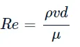
=1.225 x 6 x 0.166/1.796e-5
= 68184.866
Re > 10,000
so it is a turbulant flow
2) Nusselt number

`.023 x 68184.866^0.8 x 0.746^0.`
`169.3082`
3) Calculation of heat transfer
Nu = h/(k/l)
h = Nu x (k/l)
`169.3082 x 0.0242/0.16`
`25.6078 w/m^3`
Geometry:
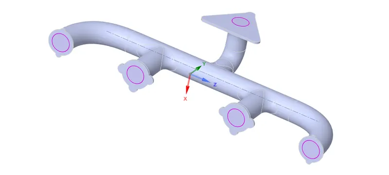
- Volume extract option from prepare is selected to extract fluid volume
- Then created a new component with both volumes(solid and fluid)
- Delete the empty components
- Share topology between solid and volume volume is enabled(pink circles ensures the share topology is enabled)
Mesh:
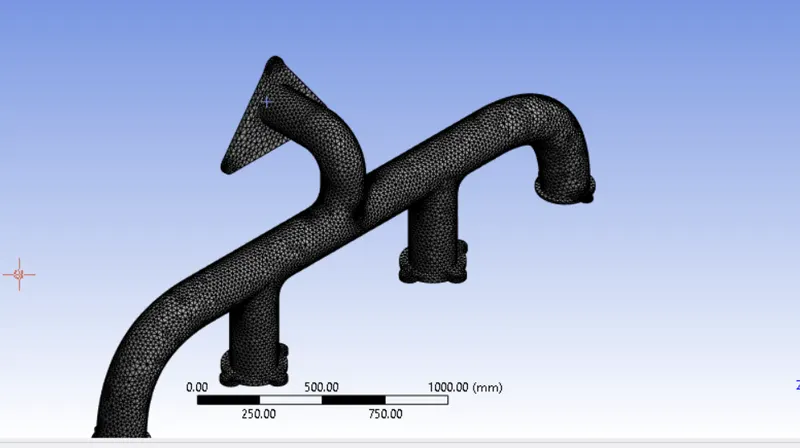
- Here we will be setting up following
- Boundaries were named as inlet,outlet,Outer-wall convection(solid volume), and the plates were named as adiabatic wall which refers it does not allow any heat transfer
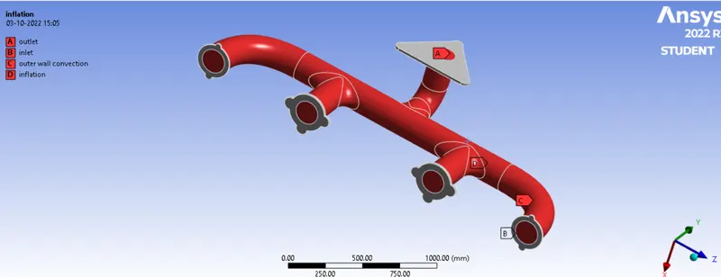
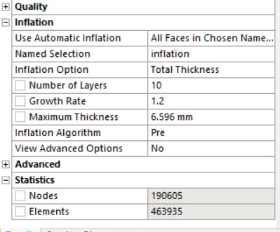
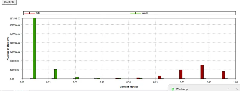
- 10 inflation layers were given
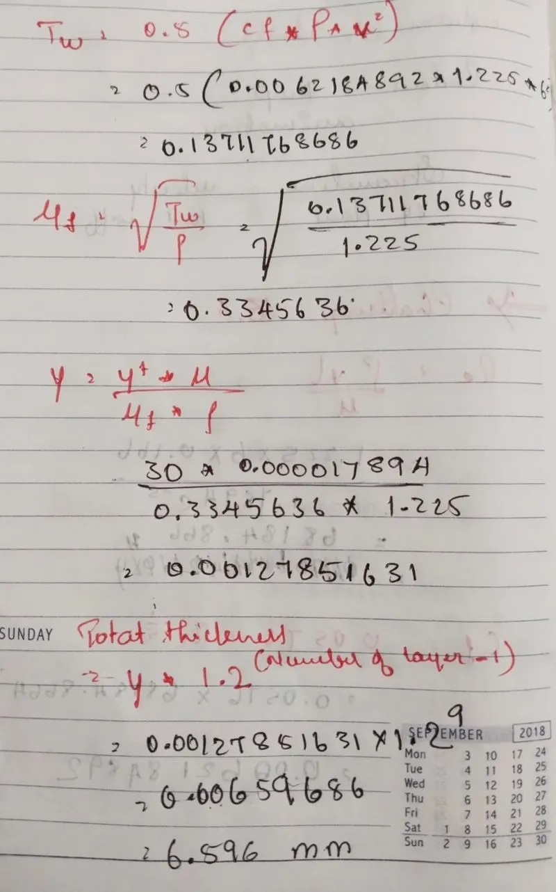
- Y+ value is set to 30 and hence the inflation layer thickness is set to 6.596 mm as total thickness
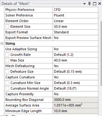
- The mesh size is given as 50mm
Setup:
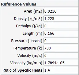
- Inlet velocity is set to 6 m/s
- Inlet Temperature is set to 700k
- On the outer wall the thermal condition is set to Convection, Heat transfer coeffecient to 20 w/m^2k, and free stream temperature as 300k
- Outlet temperature intial condition, Temperature = 300k
- Equation for energy is selected for involving the temperature into the calculation
- The viscous model is set to K-epsilon invloving 2 equations as our reynolds number exeeds 10000 we can say that it is a turbulent flow.
- Materials is set to air and aluminium for fluid and solid respectively
- I've defined to plot area weighted y-plus values , Nusselt number and heat transfer coeffecient
- In the reference values I,ve set the values as follows
- Coupled solution method is used
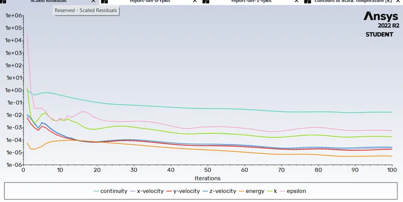
- And then for solving I,ve given 300 iteration with hybrid initialisation
Results:
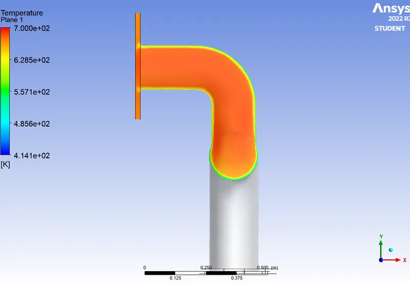
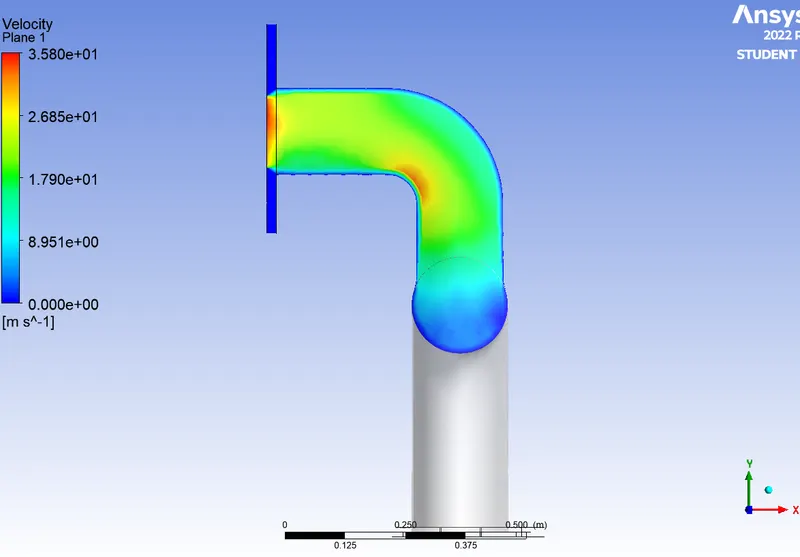
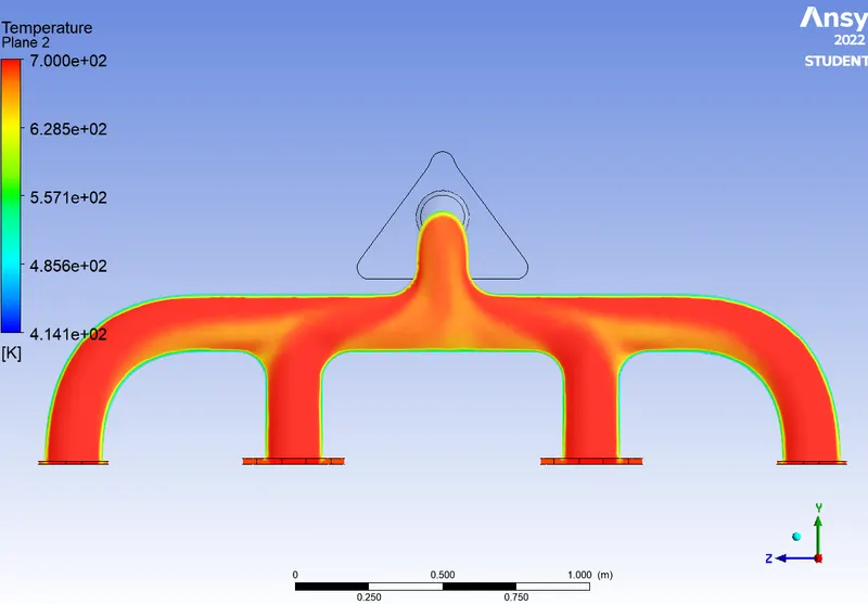
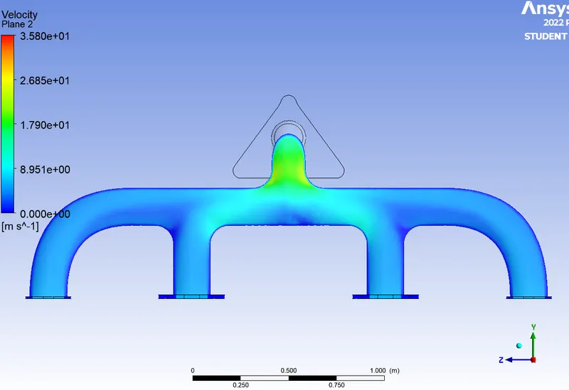
Observations:
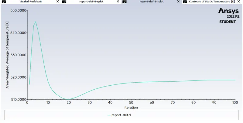
- Solution convergancy can easily be detected by looking at outlet temperature plot
- The obtained y=plus values is in range of 30-500, hence this approach is valid
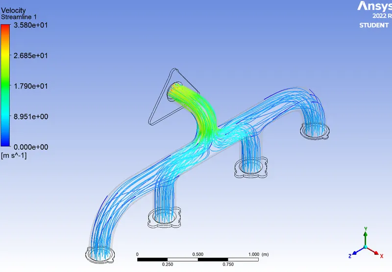
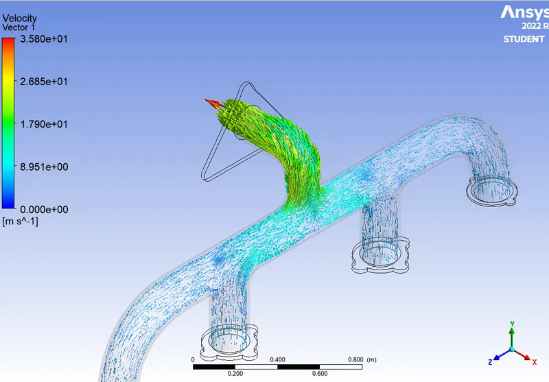
- It was observed that the velocity is higher at a point in bend(red point in velocity contour) of outlet pipe and since the velocity is higher there the heat transfer rate will also be higher at that point
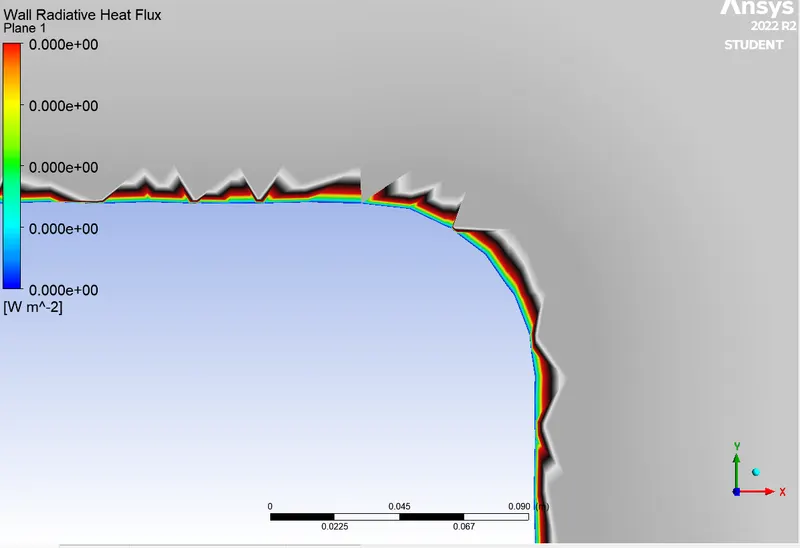
- The wall heat transfer coefficient is specificallly made for walls only
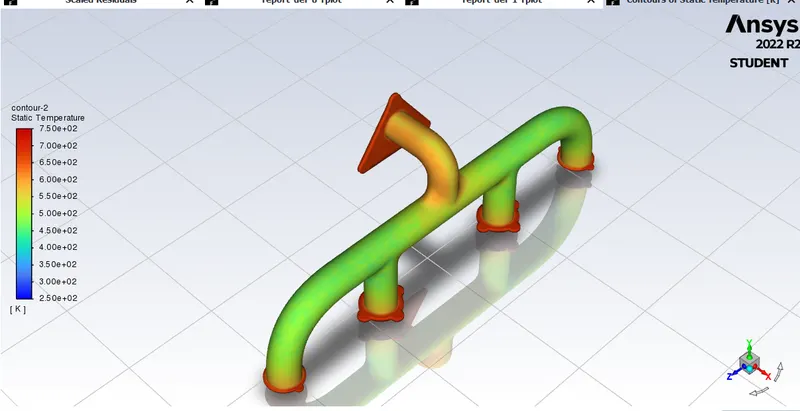
- At the temperature contour the temperature at the walls is less due to the fact that convective heat transfer has occured
- There was no much of difference spotted comparing both cases, there was only a little change in the values obtained
Discussion:
In second & third image of velocity distribution, the maximum velocity can be seen in the red color near the turining where pressure has been dropped due to sudden turn in profile & following to the maximum velocity area, low pressure area has been build up.
In similar way, in first image, the low pressure area has been seen in dark blue between the ports & low temperature can be seen at the same place in temperature distribution graph. The temperature starts dropping towards reaching the outlet of exhaust port because of the heat is transferring from the exhaust port walls & also the air from the low pressure areas in the exhaust port where air with less temperature mixed up with the hot air.
In last two images, the heat transfer coefficient has been shown. The heat transfer coefficient only visible in the first layer of the inflation layers. Thats why, in second image, the area has been zoomed to make it visible.
References:
1. https://skill-lync.com/knowledgebase/what-is-yplus
2. https://www.thermopedia.com/content/790/
3. https://www.simscale.com/docs/analysis-types/conjugate-heat-transfer-analysis/