Week 4.1 - Genetic Algorithm

1. The algorithm begins by creating a random initial population.

2. The algorithm then creates a sequence of new populations. At each step, the algorithm uses the individuals in the current generation to create the next population. To create the new population, the algorithm performs the following steps:

   • Scores each member of the current population by computing its fitness value. These values are called the raw fitness scores.

   • Scales the raw fitness scores to convert them into a more usable range of values. These scaled values are called expectation values.

   • Selects members, called parents, based on their expectation.

   • Some of the individuals in the current population that have lower fitness are chosen as elite. These elite individuals are passed to the next population.

   • Produces children from the parents. Children are produced either by making random changes to a single parent—mutation—or by combining the vector entries of a pair of parents—crossover.

   • Replaces the current population with the children to form the next generation.

3. The algorithm stops when one of the stopping criteria is met.

The genetic algorithm uses the following options to determine when to stop. See the default values for each option by running opts = optimoptions('ga').

The algorithm stops as soon as any one of these conditions is met.

STEPWISE EXPLANATION OF GA

Initial Population

The algorithm begins by creating a random initial population, as shown in the following figure.

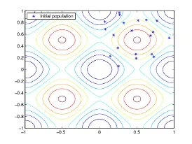
In this example, the initial population contains 20 individuals. Note that all the individuals in the initial population lie in the upper-right quadrant of the picture, that is, their coordinates lie between 0 and 1. For this example, the InitialPopulationRange option is [0;1].

If you know approximately where the minimal point for a function lies, you should set InitialPopulationRange so that the point lies near the middle of that range. For example, if you believe that the minimal point for Rastrigin's function is near the point [0 0], you could set InitialPopulationRange to be [-1;1]. However, as this example shows, the genetic algorithm can find the minimum even with a less than optimal choice for InitialPopulationRange.

Creating the Next Generation

At each step, the genetic algorithm uses the current population to create the children that make up the next generation. The algorithm selects a group of individuals in the current population, called parents, who contribute their genes—the entries of their vectors—to their children. The algorithm usually selects individuals that have better fitness values as parents. You can specify the function that the algorithm uses to select the parents in the SelectionFcn option.

The genetic algorithm creates three types of children for the next generation:

The following schematic diagram illustrates the three types of children.

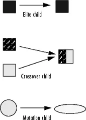
Mutation and crossover explains how to specify the number of children of each type that the algorithm generates and the functions it uses to perform crossover and mutation.

The following sections explain how the algorithm creates crossover and mutation children.

Crossover Children

The algorithm creates crossover children by combining pairs of parents in the current population. At each coordinate of the child vector, the default crossover function randomly selects an entry, or gene, at the same coordinate from one of the two parents and assigns it to the child. For problems with linear constraints, the default crossover function creates the child as a random weighted average of the parents.

IMPORTENT NOTE

GA or genatic algorithm is designed to minimize a given function. Hence to maximize the optimization problem we have incorporated -ve sign in the function f in the file staligmate.The function is attached below for references.

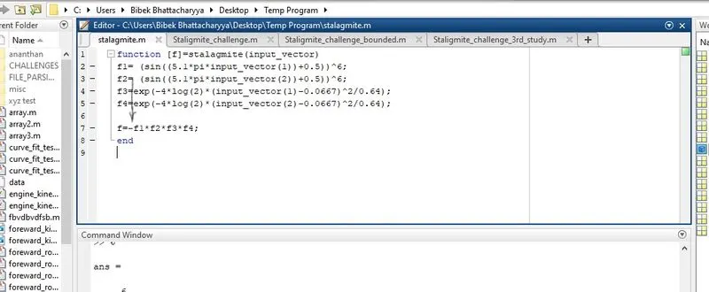
THE FUNCTION PROGRAM HAVE BEEN ATTACHED BELOW WITH COMMENTS FOR FURTHER REFERENCE.

function [f]=stalagmite(input_vector)%STALAGMITE IS THE FUNCTION NAME
f1= (sin((5.1*pi*input_vector(1))+0.5))^6;%EQUATION 1
f2= (sin((5.1*pi*input_vector(2))+0.5))^6;%EQUATION 2
f3=exp(-4*log(2)*(input_vector(1)-0.0667)^2/0.64);%EQUATION 3
f4=exp(-4*log(2)*(input_vector(2)-0.0667)^2/0.64);%EQUATION4

f=-f1*f2*f3*f4;%FUNCTION f WITH A NEGETIVE SIGN TO MAXIMIZE THE PROBLEM FINDING GLOBAL MAXIMA AS ga FINDS GLOBAL MINIMA
end

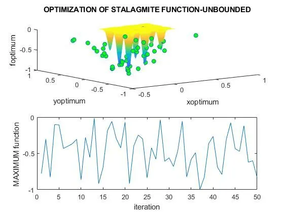
CASE 1 FOR UNBOUNDED STALAGMITE FUNCTION IS ATTACHED BELOW

clear all
close all
clc

x=linspace(0,0.6,150)%CREATING THE VALUES OF X
y=linspace(0,0.6,150)%CREATING THE VALUES FOR Y

[xx yy]=meshgrid(x,y);%CREATING MESH GRID TO FORM A 2D ARRAY

%unbounded case
for i=1:length(xx);%this means  iteration continues from 1 to 150
   for j=1:length(yy)%this means  iteration continues from 1 to 150
       input_vector(1)=xx(i,j);%this selects the x element from 2D array from ith row and jth column
       input_vector(2)=yy(i,j);%this selects the y element from 2D array from ith row and jth column
       f(i,j)=stalagmite(input_vector);%here f(i,j) means the function value of the ith row and jth column computed on basis of stalagmite function
   end
end

 
  
  numcases=50;%this 50 is the number of our search space
  tic%needed to study the simulation time
  for j=1:numcases%here we are iterating for 50 times
      [input,fopt(j)]=ga(@stalagmite,2);%it is the syntax for ga to store the two independent variable in 'input' & the function output in fopt
      xopt(j)=input(1);%since input has two colums we are seperating ot the xopt and y opt
      yopt(j)=input(2);%since input has two colums we are seperating ot the xopt and y opt
  end 
  study_1=toc%needed to record the simulation time
  %saving the figure
  figure(1)
  subplot(2,1,1)%making 2 plots in one figure window
  plot3(xopt,yopt,fopt,'o','markerfacecolor','g')%we use plot 3 command to plot 3 variables 
  title('OPTIMIZATION OF STALAGMITE FUNCTION')
  xlabel('xoptimum')%labeling
  ylabel('yoptimum')%labeling
  zlabel('foptimum')%labeling
  hold on 
 surf(xx,yy,f)
  shading interp%shading the surface areas
  hold off
  subplot(2,1,2)%ploting the second figure in figure window
  plot(fopt)
  xlabel('iteration')%labeling
  ylabel('MAXIMUM function ')%labeling
  
   

THE FIGURE FOR CASE 1 IS ATTACHED BELOW

CASE 2 FOR BOUNDED STALAGMITE FUNCTION IS ATTACHED BELOW

clear all
close all
clc

x=linspace(0,0.6,150)%CREATING THE VALUES OF X
y=linspace(0,0.6,150)%CREATING THE VALUES FOR Y

[xx yy]=meshgrid(x,y);%CREATING MESH GRID TO FORM A 2D ARRAY

%unbounded case
for i=1:length(xx);%this means  iteration continues from 1 to 150
   for j=1:length(yy)%this means  iteration continues from 1 to 150
       input_vector(1)=xx(i,j);%this selects the x element from 2D array from ith row and jth column
       input_vector(2)=yy(i,j);%this selects the y element from 2D array from ith row and jth column
       f(i,j)=stalagmite(input_vector);%here f(i,j) means the function value of the ith row and jth column computed on basis of stalagmite function
   end
end
 
  
  numcases=50;
  tic%needed to study the simulation time
  for j=1:numcases
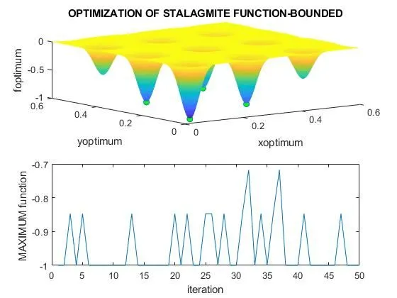
      [input,fopt(j)]=ga(@stalagmite,2,[],[],[],[],[0;0],[0.6;0.6]);
      xopt(j)=input(1);
      yopt(j)=input(2);
  end 
  study2_time=toc%needed to record the simulation time
   %saving the figure
  figure(1)
  subplot(2,1,1)%making 2 plots in one figure window
  plot3(xopt,yopt,fopt,'o','markerfacecolor','g')%we use plot 3 command to plot 3 variables 
  title('OPTIMIZATION OF STALAGMITE FUNCTION')
  xlabel('xoptimum')%labeling
  ylabel('yoptimum')%labeling
  zlabel('foptimum')%labeling
  hold on 
 surf(xx,yy,f)
  shading interp%shading the surface areas
  hold off
  subplot(2,1,2)%ploting the second figure in figure window
  plot(fopt)
  xlabel('iteration')%labeling
  ylabel('MAXIMUM function ')%labeling
 
  
   

THE FIGURE FOR CASE 2 IS ATTACHED BELOW

CASE 3 FOR POPULATION VARIATION STALAGMITE FUNCTION IS ATTACHED BELOW

clear all
close all
clc

x=linspace(0,0.6,150)%CREATING THE VALUES OF X
y=linspace(0,0.6,150)%CREATING THE VALUES FOR Y

[xx yy]=meshgrid(x,y);%CREATING MESH GRID TO FORM A 2D ARRAY

%unbounded case
for i=1:length(xx);%this means  iteration continues from 1 to 150
   for j=1:length(yy)%this means  iteration continues from 1 to 150
       input_vector(1)=xx(i,j);%this selects the x element from 2D array from ith row and jth column
       input_vector(2)=yy(i,j);%this selects the y element from 2D array from ith row and jth column
       f(i,j)=stalagmite(input_vector);%here f(i,j) means the function value of the ith row and jth column computed on basis of stalagmite function
   end
end
 
  
  numcases=50;
  
  options=optimoptions('ga');
  options=optimoptions(options,'populationsize',170)
  
  tic%needed to study the simulation time
  for j=1:numcases
      [input,fopt(j)]=ga(@stalagmite,2,[],[],[],[],[0;0],[0.6;0.6],[],[],options);
      xopt(j)=input(1);
      yopt(j)=input(2);
  end 
  study3_time=toc%needed to record the simulation time
  
   %saving the figure
  figure(1)
  subplot(2,1,1)%making 2 plots in one figure window
  plot3(xopt,yopt,fopt,'o','markerfacecolor','g')%we use plot 3 command to plot 3 variables 
  title('OPTIMIZATION OF STALAGMITE FUNCTION-POPULATION VARIATION')
  xlabel('xoptimum')%labeling
  ylabel('yoptimum')%labeling
  zlabel('foptimum')%labeling
  hold on 
 surf(xx,yy,f)
  shading interp%shading the surface areas
  hold off
  subplot(2,1,2)%ploting the second figure in figure window
  plot(fopt)
  xlabel('iteration')%labeling
  ylabel('MAXIMUM function ')%labeling
  
  
   

THE FIGURE FOR CASE 3 IS ATTACHED BELOW:

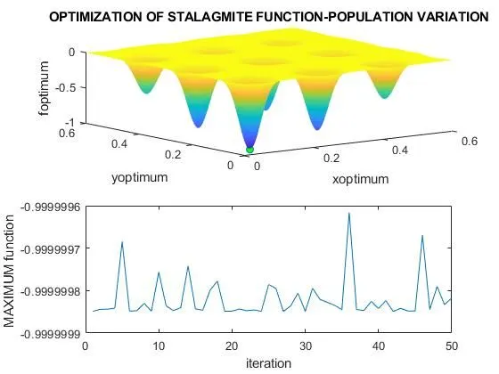
CONCLUSION:-HENCE BY SERIES OF THESE EXPERIMENTS AND ITERATION THE GLOBAL MAXIMA HAVE BEEN FOUND OUT