Week 5.1 - Mid term project - Solving the steady and unsteady 2D heat conduction problem

STEADY STATE PROBLEM (EXPLICIT)

AIM:

Steady state analysis

BOUNDARY CONDITION:

Top Boundary = 600 K

Bottom Boundary = 900 K

Left Boundary = 400 K

Right Boundary = 800 K

ITERATIVE METHODS TO USE:

We will implement the following methods for solving implicit equations.

1. Jacobi.

2. Gauss-seidel.

3. Successive over-relaxation.

BEFORE WE PROCEED LET US CHECK HOW THE DERIVATION GOES ON THEN WE CAHN EASILY MOVE ON WITH THE CODING SEGMENT IN MATLAB.

THE DETAILED DERIVATION IS USED BELOW:

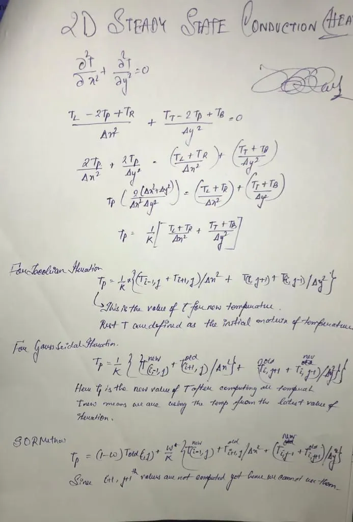
LET US FIRST UNDERSTAND WHAT HAPPENS IN HERE .

1. JACOBI METHOD-IN JACOBI WE ARE COMPUTING THE TEMPERATURE AT THE GRIDPOINTS HAVING A PREDETERMINED GUESS VALUE LIKE 300K AND SLOWLY MOVING TOWARDS CONVERGENCE . ie GRADUALLY THE TEMPERATURE IS DIFFUSING THROUGH THE WHOLE PLATE. AS WE USE JACOBI METHOD WE COMPUTE THE VALUE OF ONE POINT BASED ON THE ASSUMPTION AT THE BEGINNING OF THE PROBLEM. EXAMPLE IS DEFINED IN THE IMAGE BELOW.
   
   
   
   
   
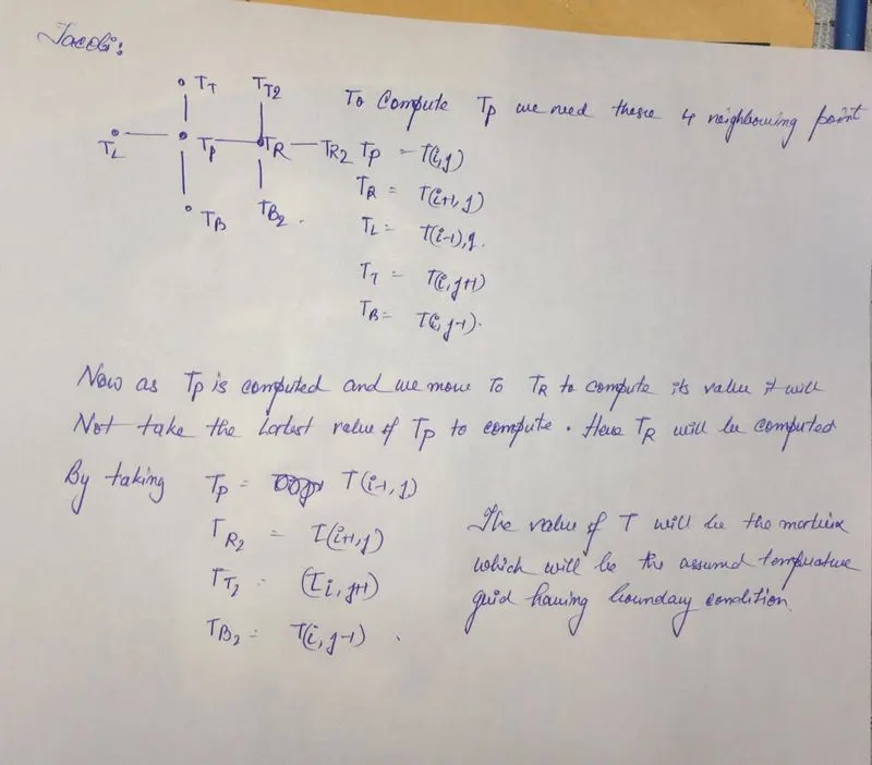
   1. LET US SEED NOW HOW THE CODE GOES ON.

   clear all
   close all
   clc

   n=10; Here we are specifying the numbe of node points and we will us this node number to define ranges of temperatuire of the gridpoints.
   l=5; Specifying the length of grid of x and y axis.
   b=l;
   x=linspace(0,l,n); Splitting x and y xis in n number of gridpoints.
   y=linspace(0,b,n);
   dx=x(2)-x(1); Defining the dx and dy value
   dy=dx;

   T=300*ones(n,n); Defining the size of matrix T which contains the temperature values.

   Defining the boundary condition
   T(1,1:n)=600;
   T(1:n,1)=400;
   T(n,1:n)=900;
   T(1:n,n)=800;

   T(1,1)=500;
   T(1,n)=700;
   T(n,1)=650;
   T(n,n)=850;

   %defining SOR factor
   w=1.2;

   %updating the T values and creating a copy of the matrix.
   Told=T;
   tol=1e-4; HERE TOL REFERS TO THE MAX ERROR TERM THE PROGRAM SHOULD HAVE . ALL OTHER ERRORS SHOULD BE LESS THAN THIS ERROR.
   error=9e9;

   
   %this is the iteration specifier
   %1=solving by Jacobian method
   %2=solving by Gauss_Geidal method
   %3=solving by SOR method
   iterative_solver=1

   HERE WE AERE SPECIFYING BY NUMBER 1 2 AND 3 WHICHJ SLOVER TO USE. IT HAS 3 SOLVERS IN THIS PROGRAM.

   If you go through the simpification process of discreetization and follow the attached document you will find out that we have assumed k as the product and division of the following terms.
   k=(2*(dx^2+dy^2))/((dx^2)*(dy^2))

   clear all
   close all
   clc
   
   n=10; %here we are specifying the numbe of node points and we  will us this node number to define ranges of the temperatuire of the gridpoints. 
   l=5; %specifying the length of grid of x and y axis.
   b=l;
   x=linspace(0,l,n); %splitting x and y xis in n number of gridpoints.
   y=linspace(0,b,n);
   dx=x(2)-x(1); %defining the dx and dy  value
   dy=dx;
   
   T=300*ones(n,n); %defining the size of matrix T which contains the temperature values.
   
   %defining the boundary condition
   T(1,1:n)=600;
   T(1:n,1)=400;
   T(n,1:n)=900;
   T(1:n,n)=800;
   
   T(1,1)=500;
   T(1,n)=700;
   T(n,1)=650;
   T(n,n)=850;
   
   %defining SOR factor
    w=1.2;
   
    %updating the T values and creating a copy of the matrix.
   Told=T;
   tol=1e-4;
   error=9e9;
   
   
   %this is the iteration specifier
   %1=solving by Jacobian method
   %2=solving by Gauss_Geidal method
   %3=solving by SOR method
   iterative_solver=1
   
   %if you go through the simpification process of discreetization and follow
   %the attached document you will find out that we have assumed k as the
   %product and division of the following terms.
   k=(2*(dx^2+dy^2))/((dx^2)*(dy^2))

   SINCE WE ARE TALKING ABOUT JACOBIAN LETS FIRST PROGRAM FOR THE JACOBIAN ITERATIVE SOLVER.

   tic :Tic toc commands are used to record the time each iterative solver is taking to converge.
   if iterative_solver==1 Specifying which solver is this.
   jacobi_iter=1 This is the iteration counter which gets updated at the end of each cycle.
   
   Here we are usng a while loop to specify how long the iteration should run. As long as the error value is greater than the tolerance value the loop should go on. The moment the error term is leass than tolerance value the solution converges.
   
   while error>tol
   
   
   for i=2:n-1 %HERE WE ARE SPECIFYING THAT THE LOOP MUST RUN FOR N-1 VALUES FOR NODES N IN X AXIS
   for j=2:n-1 %HERE WE ARE SPECIFYING THAT THE LOOP MUST RUN FOR N-1 VALUES FOR NODES N IN Y AXIS
   
   T(i,j)=(1/k)*(((Told(i-1,j)+Told(i+1,j))/dx^2)+((Told(i,j-1)+Told(i,j+1))/dy^2)) %HERE WE ARE IMPLEMENTING THE JACOBIAN FORMULAE. PLEASE REFER TO THE ATTACHED DERIVATION.

   
   end
   end
   error=max(max(abs(Told-T))) HERE WE ARE CALCULATION THE MAXIMUM POSSIBLE ERROR BETWEEN THE CURRENT TEMPERATURE MATRIX AND THE MATRIX IN THE PREVIOUS TIMESTEP

   THIS WILL HELP US TO RUN THE WHILE LOOP. AS LONG AS THE ERROR IS > THAN TOL VALUE THEN THE LOOP WILL RUN. THIS IS OUR CONVERGENCE CRITERIA.
   Told=T; HERE WE UPDATE THE MATRIX TO BE USED IN THE NEXT WHILE LOOP OR NEXT ITEERATION.
   jacobi_iter=jacobi_iter+1 %THIS IS THE ITERATION COUNTER. AS THE WHILE LOOP PROCEEDS THIS LOOP VALUE INCREASES BY WITH EACH ITRTATION.
   figure(1)
   c=contourf(x,y,T,'showtext','on') %HERE WE ARE PLOTTING X AND Y AS A FUNCTION OF THE TEMPERATURE. IT SHOWS THE DISTRIBUTION OF TEMPERATURE AS THE SYSTEM APPROACHES STEADY STATE.
   colormap(jet)
   colorbar %IT SHOWS WHICH PART HAVE WHAT TEMPERATURE.
   %jacobi iter for 10 nodes 205
   
   end
   end

   HERE IS THE CODE ATTACHED BELOW.

   tic %tic toc commands are used to record the time each iterative solver is taking to converge.
     if iterative_solver==1 %specifying which solver is this.
        jacobi_iter=1 %this is the iteration counter which gets updated at the end of each cycle.
      
        %here we are usng a while loop to specify how long the iteration
        %should run. As long as the error value is greater than the tolerance
        %value the loop should go on. The moment the error term is leass than
        %tolerance value the solution converges.
        
        while error>tol
            
            
       for i=2:n-1
           for j=2:n-1
               
               T(i,j)=(1/k)*(((Told(i-1,j)+Told(i+1,j))/dx^2)+((Told(i,j-1)+Told(i,j+1))/dy^2))
   
               
           end
       end
       error=max(max(abs(Told-T)))
       Told=T;
        jacobi_iter=jacobi_iter+1
        figure(1)
        c=contourf(x,y,T,'showtext','on')
        set(gca,'YDIR','reverse')
        colormap(jet)
        colorbar
        %jacobi iter for 10 nodes 205
      
   end
     end
   

   THE SOLUTION WE GET FROM JACOBIAN METHOD GIVES US RESULT AFTER 205 ITERATION. HENCE IT TAKES SOME TIME TO CONVERGE. THE RESULT OF THE CONVERGENCE IS ATTACHED BELOW.

   THE SOLUTION TIME IS 22.3985 SEC.

   

2. GAUSS SEIDAL METHOD:IN THIS METHOD WE ARE GOING TO COMPUTE THE VALUE OF A PARTICULAR POINT BASED ON THE OUTPUT OF THE PREVIOUSLY CALCULATED NODE.THE DETAIL IS EXPLAIENED BELOW.
   
   
   
   
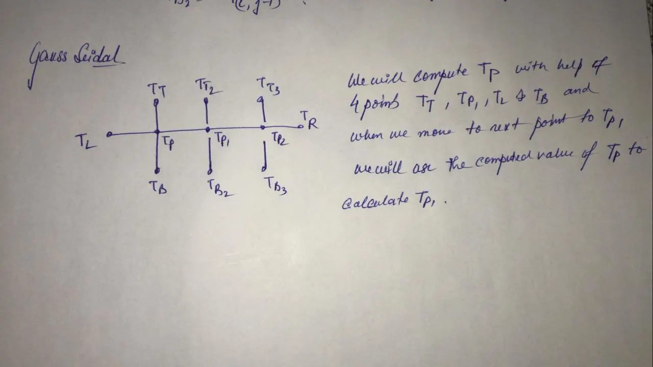
   SINCE WE ARE TALKING ABOUT GAUSS SEIDAL LETS FIRST PROGRAM FOR THE GAUSS SEIDAL ITERATIVE SOLVER.
   
   %using gs method
   
   
   tic Tic toc commands are used to record the time each iterative solver is taking to converge.
   if iterative_solver==1 Specifying which solver is this.
   gs_iter=1 This is the iteration counter which gets updated at the end of each cycle.
   while error>tol Here we are usng a while loop to specify how long the iteration should run. As long as the error value is greater than the tolerance value the loop should go on. The moment the error term is leass than tolerance value the solution converges.
   for i=2:n-1 %HERE WE ARE SPECIFYING THAT THE LOOP MUST RUN FOR N-1 VALUES FOR NODES N IN X AXIS
   for j=2:n-1 %HERE WE ARE SPECIFYING THAT THE LOOP MUST RUN FOR N-1 VALUES FOR NODES N IN Y AXIS
   
   T(i,j)=(1/k)*(((T(i-1,j)+Told(i+1,j))/dx^2)+((T(i,j-1)+Told(i,j+1))/dy^2))
   
   
   end
   end
   

   error=max(max(abs(Told-T))) HERE WE ARE CALCULATION THE MAXIMUM POSSIBLE ERROR BETWEEN THE CURRENT TEMPERATURE MATRIX AND THE MATRIX IN THE PREVIOUS TIMESTEP

   THIS WILL HELP US TO RUN THE WHILE LOOP. AS LONG AS THE ERROR IS > THAN TOL VALUE THEN THE LOOP WILL RUN. THIS IS OUR CONVERGENCE CRITERIA.
   Told=T; HERE WE UPDATE THE MATRIX TO BE USED IN THE NEXT WHILE LOOP OR NEXT ITEERATION.
   jacobi_iter=jacobi_iter+1 %THIS IS THE ITERATION COUNTER. AS THE WHILE LOOP PROCEEDS THIS LOOP VALUE INCREASES BY WITH EACH ITRTATION.
   figure(2)
   c=contourf(x,y,T,'showtext','on') %HERE WE ARE PLOTTING X AND Y AS A FUNCTION OF THE TEMPERATURE. IT SHOWS THE DISTRIBUTION OF TEMPERATURE AS THE SYSTEM APPROACHES STEADY STATE.

   set(gca,'YDIR','reverse')
   xlabel('X AXIS') %SPECIFYING X AND Y AXIS
   ylabel('Y AXIS')
   title('GAUSS SEIDAL ITERATIVE SOLVER')
   colormap(jet) IT SHOWS EHICH PART HAVE WHAT TEMPERATURE.
   colorbar
   nd
   end
   gs_timer=toc %gs_iter for 10 nodes =111
   %13.904 TIME.
   
   HERE IS THE CODE ATTACHED BELOW.
   
   

     %using gs method
     if iterative_solver==2
        gs_iter=1
   while error>tol
       
       for i=2:n-1
           for j=2:n-1
               
               T(i,j)=(1/k)*(((T(i-1,j)+Told(i+1,j))/dx^2)+((T(i,j-1)+Told(i,j+1))/dy^2))
              
               
           end
       end
       error=max(max(abs(Told-T)))
       Told=T;
        gs_iter=gs_iter+1
        figure(2)
        c=contourf(x,y,T,'showtext','on')
        set(gca,'YDIR','reverse')
         xlabel('X AXIS')
           ylabel('Y AXIS')
           title('GAUSS SEIDAL ITERATIVE SOLVER')
        colormap(jet)
        colorbar
        %gs_iter for 10 nodes =111
        %13.904 TIME
      
   end
     end
   gs_timer=toc

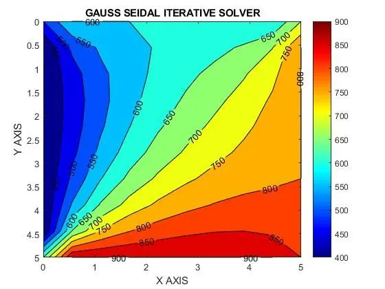
   THE SOLUTION WE GET FROM GAUSS SEIDAL METHOD GIVES US RESULT AFTER 111 ITERATION. HENCE IT TAKES SOME LESS TIME TO CONVERGE. THE RESULT OF THE CONVERGENCE IS ATTACHED BELOW.THE SOLUTION TIME IS 13.904 SEC. THUS WE CAN SEE AND COMPARE THAT USING THE VALUE FROM THE LAST STEP GIVES US AN EDGE OVER USING REPEATED OLD VALUES. THE NUMBER OF ITERATION DECREASES, SOLUTION CONVERGES MUCH EASILY AND TAKES MUCH LESS TIME.
   
   
   
   

3. SUCCESSIVE OVER RELAXATION METHOD: IN SUCCESSIVE RELAXATION WE ADD A PARTICULAR FACTOR GREATER THAN 1 TO MAKE IT OVER RELAXATED. THIS FACTOR IF 1 WILL BE EQUAL TO GS METHOD.BUT OUR MAIN AIM IS TO SCALE THE EQUATION IN SUCH A WAY THAT IT GIVES MOST ACCURATE YET LEAST ITERATION.
   
   THE CODE IS AS FOLLOWS. EVERYTHING IS SIMILAR JUST THE w IS USED HAVING A VALUE OF 1.2.
   

   tic
   if iterative_solver==3
        sor_iter=1
   while error>tol
       
       for i=2:n-1
           for j=2:n-1
              
               
               T(i,j)=(1-w)*Told(i,j)+(w/k)*(((T(i-1,j)+Told(i+1,j))/dx^2)+((T(i,j-1)+Told(i,j+1))/dy^2));
                
               
           end
       end
       error=max(max(abs(Told-T)))
       Told=T;
        sor_iter=sor_iter+1
        figure(2)
        c=contourf(x,y,T)
        c=contourf(x,y,T,'showtext','on')
        set(gca,'YDIR','reverse')
         xlabel('X AXIS')
           ylabel('Y AXIS')
           title('SOR ITERATIVE SOLVER')
        colormap(jet)
        colorbar
        %sor_iter for 10 nodes =75
      
   end
     end
   sor_time=toc %7.9827 SEC
   

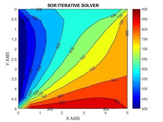
   THE SOLUTION WE GET FROM SOR METHOD GIVES US RESULT AFTER 75 ITERATION. HENCE IT TAKES SOME LESS TIME TO CONVERGE THAN GAUSS SEIDAL METHOD . THE RESULT OF THE CONVERGENCE IS ATTACHED BELOW.THE SOLUTION TIME IS 7.9827 SEC. THUS WE CAN SEE AND COMPARE THAT USING THE VALUE w GIVES US AN EDGE OVER USING REPEATED OLD VALUES. THE NUMBER OF ITERATION DECREASES, SOLUTION CONVERGES MUCH EASILY AND TAKES MUCH LESS TIME.
   
   
   
   
   
   THE WHOLE CODE IS ATTACHED BELOW.
   

   clear all
   close all
   clc
   
   n=10; %here we are specifying the numbe of node points and we  will us this node number to define ranges of the temperatuire of the gridpoints. 
   l=5; %specifying the length of grid of x and y axis.
   b=l;
   x=linspace(0,l,n); %splitting x and y xis in n number of gridpoints.
   y=linspace(0,b,n);
   dx=x(2)-x(1); %defining the dx and dy  value
   dy=dx;
   
   T=300*ones(n,n); %defining the size of matrix T which contains the temperature values.
   
   %defining the boundary condition
   T(1,1:n)=600;
   T(1:n,1)=400;
   T(n,1:n)=900;
   T(1:n,n)=800;
   
   T(1,1)=500;
   T(1,n)=700;
   T(n,1)=650;
   T(n,n)=850;
   
   %defining SOR factor
    w=1.2;
   
    %updating the T values and creating a copy of the matrix.
   Told=T;
   tol=1e-4;
   error=9e9;
   
   
   %this is the iteration specifier
   %1=solving by Jacobian method
   %2=solving by Gauss_Geidal method
   %3=solving by SOR method
   iterative_solver=1
   
   %if you go through the simpification process of discreetization and follow
   %the attached document you will find out that we have assumed k as the
   %product and division of the following terms.
   k=(2*(dx^2+dy^2))/((dx^2)*(dy^2))
   
   %using jacobian method
   tic %tic toc commands are used to record the time each iterative solver is taking to converge.
     if iterative_solver==1 %specifying which solver is this.
        jacobi_iter=1 %this is the iteration counter which gets updated at the end of each cycle.
      
        %here we are usng a while loop to specify how long the iteration
        %should run. As long as the error value is greater than the tolerance
        %value the loop should go on. The moment the error term is leass than
        %tolerance value the solution converges.
        
        while error>tol
            
            
       for i=2:n-1
           for j=2:n-1
               
               T(i,j)=(1/k)*(((Told(i-1,j)+Told(i+1,j))/dx^2)+((Told(i,j-1)+Told(i,j+1))/dy^2))
   
               
           end
       end
       error=max(max(abs(Told-T)))
       Told=T;
        jacobi_iter=jacobi_iter+1
        figure(1)
        c=contourf(x,y,T,'showtext','on')
        set(gca,'YDIR','reverse')
        xlabel('X AXIS')
           ylabel('Y AXIS')
           title('JACOBIAN ITERATIVE SOLVER')
        colormap(jet)
        colorbar
        %jacobi iter for 10 nodes 208
      %24.7035 SEC
   end
     end
     jacobian_timer=toc
     
     
     
     tic
     %using gs method
     if iterative_solver==2
        gs_iter=1
   while error>tol
       
       for i=2:n-1
           for j=2:n-1
               
               T(i,j)=(1/k)*(((T(i-1,j)+Told(i+1,j))/dx^2)+((T(i,j-1)+Told(i,j+1))/dy^2))
              
               
           end
       end
       error=max(max(abs(Told-T)))
       Told=T;
        gs_iter=gs_iter+1
        figure(2)
        c=contourf(x,y,T,'showtext','on')
        set(gca,'YDIR','reverse')
         xlabel('X AXIS')
           ylabel('Y AXIS')
           title('GAUSS SEIDAL ITERATIVE SOLVER')
        colormap(jet)
        colorbar
        %gs_iter for 10 nodes =112
        %13.966 TIME
      
   end
     end
   gs_timer=toc
   tic
   if iterative_solver==3
        sor_iter=1
   while error>tol
       
       for i=2:n-1
           for j=2:n-1
              
               
               T(i,j)=(1-w)*Told(i,j)+(w/k)*(((T(i-1,j)+Told(i+1,j))/dx^2)+((T(i,j-1)+Told(i,j+1))/dy^2));
                
               
           end
       end
       error=max(max(abs(Told-T)))
       Told=T;
        sor_iter=sor_iter+1
        figure(3)
        c=contourf(x,y,T,'showtext','on')
        set(gca,'YDIR','reverse')
         xlabel('X AXIS')
           ylabel('Y AXIS')
           title('SOR ITERATIVE SOLVER')
        colormap(jet)
        colorbar
        %sor_iter for 10 nodes =76
      
   end
     end
   sor_time=toc %8.7207
   
   
   
   
   
   
   
   
   
   
   
   
   
   
   
   
   
   
   
   
   
   
   
   
   
   
   
   
   
   

THE CONCLUSION DRAWN FROM THE 3 ITERATIVE METHOD OF STEADY STATE ARE AS FOLLOWS.

STEADY STATE ITERATIVE METHOD	NUMBER OF ITERATION	CONVERGENCE TIME
1.JACOBI METHOD	208	24.7035
2.GAUSS SEIDAL METHOD	112	13.966
3.SOR METHOD	76	8.7207

CONCLUSION: HENCE THE CONCLUSION THAT CAN BE DRAWN FROM THE STEADY STATE EQUATIONS AND ITERATIONS IS THAT THE ITERATION IS IN ORDER JACOBI>GAUSS SEIDAL>SOR & THE SWIFTNESS OF EQUATION SOLVING IS IN THE ORDER SOR>GAUSS-SEIDAL>JACOBI.

TRANSIENT STATE PROBLEM (EXPLICIT)

AIM:

TRANSIENT STATE EXPLICIT ANALYSIS.

BOUNDARY CONDITION:

Top Boundary = 600 K

Bottom Boundary = 900 K

Left Boundary = 400 K

Right Boundary = 800 K

BEFORE WE PROCEED LET US CHECK HOW THE DERIVATION GOES ON THEN WE CAHN EASILY MOVE ON WITH THE CODING SEGMENT IN MATLAB.

THE DETAILED DERIVATION IS USED BELOW:

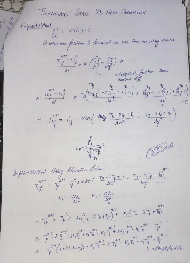
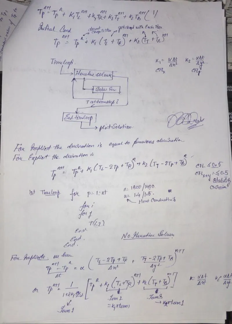
SINCE WE HAVE DERIVED THE BASICS LETS START WITH THE EXPLICIT METHOD FOR TRANSIENT HEAT TRANSFER. THE CODE GOES AS FOLLOWS.

FIRST WE DEFINE THE BASIC PARAMETERS; SUCH AS FOLOWS.

clear all
close all
clc

n=10; here we are specifying the numbe of node points and we will us this node number to define ranges of the temperatuire of the gridpoints.
l=5; specifying the length of grid of x and y axis.
b=l;
x=linspace(0,l,n); splitting x and y xis in n number of gridpoints.
y=linspace(0,b,n);
dx=x(2)-x(1); defining the dx and dy value
dy=dx;
a=1.4;
dt=1e-2;

T=300*ones(n,n); defining the size of matrix T which contains the temperature values.

defining the boundary condition
T(1,1:n)=600;
T(1:n,1)=400;
T(n,1:n)=900;
T(1:n,n)=800;

T(1,1)=500;
T(1,n)=700;
T(n,1)=650;
T(n,n)=850;

updating the T values and creating a copy of the matrix.
Told=T;

clear all
close all
clc

n=10; %here we are specifying the numbe of node points and we  will us this node number to define ranges of the temperatuire of the gridpoints. 
l=5; %specifying the length of grid of x and y axis.
b=l;
x=linspace(0,l,n); %splitting x and y xis in n number of gridpoints.
y=linspace(0,b,n);
dx=x(2)-x(1); %defining the dx and dy  value
dy=dx;
a=1.4;
dt=1e-2;

T=300*ones(n,n); %defining the size of matrix T which contains the temperature values.

%defining the boundary condition
T(1,1:n)=600;
T(1:n,1)=400;
T(n,1:n)=900;
T(1:n,n)=800;

T(1,1)=500;
T(1,n)=700;
T(n,1)=650;
T(n,n)=850;


%updating the T values and creating a copy of the matrix.
Told=T;     

NOW LET US YAKE A LOOK INTO THE FOR LOOPS.

• THE FIRST FOR LOOP IS FOR THE TIME STEPS ALSO KNOWN AS THE LOOP FOR TIME MARCHING
• THIS REPRESENTS THAT IT HAS TO RUN FOR 1400 STEPS TO CONVERGE.
• 1400*1E-2=14 IS THE TOTAL TIME REQUIRED FOR THE SIMULATION.
• THE SECOND AND THIRD FOR LOOPS ARE FOR THE SPACEMARCHING.
• THE EQUATION T(i,j)=Told(i,j)*(1-2*k1-2*k2)+k1*(Told(i-1,j)+Told(i+1,j))+k2*(Told(i,j-1)+Told(i,j+1)); HELPS US TO FIND THE GRIDPOINTS ON THE BASIS OF PRILIMINARY Told.
• HENCE AFTER THE LOOP ENDS THE T THAT WE OBTAIN HAS TO UPDATED WITH THE Told TO RUN FOR THE SECOND TIMESTEP ITERATION. HENCE WE USE THE FOLLOWING CODE.
  

  tic  %RECORDING THE TIME TAKEN WITH TIC TOC COMMAND
        %time loop
        for p=1:1400;
      
  
  %   CALCULATING THE CFL NUMBERS
  
  k1=(a*dt)/dx^2; 
  k2=(a*dt)/dy^2;
  
  
  
  
      for i=2:n-1
          for j=2:n-1
              
          %HERE WE ARE DEFINING T AS A FUNCTION OF THE DISCRETIZED EQUATION
          %Told  REPRESENTS THE TEMP MATRIX THAT WE FORMED AT THE BEGINNING
          %THE TWO FOR LOOPS COMPUTE THE TEMP PROFILE FOR A PARTICULAT
          %TIMESTEP.
        T(i,j)=Told(i,j)*(1-2*k1-2*k2)+k1*(Told(i-1,j)+Told(i+1,j))+k2*(Told(i,j-1)+Told(i,j+1));
               
          end
      end
      
      Told=T; %THIS IS WHERE THE Told IS UPDATED WITH THE COMPUTED VALUE OF 2 FOR LOOPS.
      %THIS NEW UPDATED Told IS USED TO COMPUTE THE  TEMPERATURE OF THE
      %GRIDPOINTS IN THE NEXT TIMESTEP.
       
    
     
  end
        
  

  
  
  

THE NEXT TEP IS TO PLOT THE CONTOUR OF THE X,Y AND T IN THE FIGUER WINDOW. THE CODE IS AS FOLLOWS.

figure(1)
     c=contourf(x,y,T,'showtext','on') %THIS IS USED TO PLOT THE GRAPH IN CY PLANE WRT TEMPERATURE.
     set(gca,'YDIR','reverse')
     %LABELING  X AND Y AXIS
     xlabel('X AXIS')
        ylabel('Y AXIS')
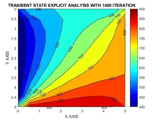
        title('TRANSIENT STATE EXPLICIT ANALYSIS WITH 1400 ITERATION')
     colormap(jet)
     colorbar
  
     transient_explicit_time=toc   %0.5100 seconds.

THE FULL CODE IS HERE ATTACHED.

clear all
close all
clc

n=10; %here we are specifying the numbe of node points and we  will us this node number to define ranges of the temperatuire of the gridpoints. 
l=5; %specifying the length of grid of x and y axis.
b=l;
x=linspace(0,l,n); %splitting x and y xis in n number of gridpoints.
y=linspace(0,b,n);
dx=x(2)-x(1); %defining the dx and dy  value
dy=dx;
a=1.4;
dt=1e-2;

T=300*ones(n,n); %defining the size of matrix T which contains the temperature values.

%defining the boundary condition
T(1,1:n)=600;
T(1:n,1)=400;
T(n,1:n)=900;
T(1:n,n)=800;

T(1,1)=500;
T(1,n)=700;
T(n,1)=650;
T(n,n)=850;


%updating the T values and creating a copy of the matrix.
Told=T;     


tic  %RECORDING THE TIME TAKEN WITH TIC TOC COMMAND
      %time loop
      for p=1:1400;
    

%   CALCULATING THE CFL NUMBERS

k1=(a*dt)/dx^2; 
k2=(a*dt)/dy^2;




    for i=2:n-1
        for j=2:n-1
            
        %HERE WE ARE DEFINING T AS A FUNCTION OF THE DISCRETIZED EQUATION
        %Told  REPRESENTS THE TEMP MATRIX THAT WE FORMED AT THE BEGINNING
        %THE TWO FOR LOOPS COMPUTE THE TEMP PROFILE FOR A PARTICULAT
        %TIMESTEP.
      T(i,j)=Told(i,j)*(1-2*k1-2*k2)+k1*(Told(i-1,j)+Told(i+1,j))+k2*(Told(i,j-1)+Told(i,j+1));
             
        end
    end
    
    Told=T; %THIS IS WHERE THE Told IS UPDATED WITH THE COMPUTED VALUE OF 2 FOR LOOPS.
    %THIS NEW UPDATED Told IS USED TO COMPUTE THE  TEMPERATURE OF THE
    %GRIDPOINTS IN THE NEXT TIMESTEP.
     
  
   
end
      
figure(1)
     c=contourf(x,y,T,'showtext','on') %THIS IS USED TO PLOT THE GRAPH IN CY PLANE WRT TEMPERATURE.
     set(gca,'YDIR','reverse')
     %LABELING  X AND Y AXIS
     xlabel('X AXIS')
        ylabel('Y AXIS')
        title('TRANSIENT STATE EXPLICIT ANALYSIS WITH 1400 ITERATION')
     colormap(jet)
     colorbar
  
     transient_explicit_time=toc   %0.5100 seconds.

THE GRAPH IS HERE AS FOLLOWS.

TRANSIENT STATE PROBLEM (IMPLICIT)

AIM:

TRANSIENT STATE EXPLICIT ANALYSIS.

BOUNDARY CONDITION:

Top Boundary = 600 K

Bottom Boundary = 900 K

Left Boundary = 400 K

Right Boundary = 800 K

ITERATIVE METHODS TO USE:

We will implement the following methods for solving implicit equations.

1. Jacobi.

2. Gauss-seidel.

3. Successive over-relaxation.

BEFORE WE PROCEED LET US CHECK HOW THE DERIVATION GOES ON THEN WE CAHN EASILY MOVE ON WITH THE CODING SEGMENT IN MATLAB.

THE DETAILED DERIVATION IS USED BELOW:

SINCE WE HAVE DERIVED THE BASICS LETS START WITH THE EXPLICIT METHOD FOR TRANSIENT HEAT TRANSFER. THE CODE GOES AS FOLLOWS.

FIRST WE DEFINE THE BASIC PARAMETERS; SUCH AS FOLOWS.

THE IMLPLICIT SCHEME MAINLY DEALS WITH THE UN-COMPUTED POINTS IN THE DOMAIN TAKING ASSUMPTIONS FROM THE POINTS IN THE GRID THAT ARE YET TO COMPUTE.

LET US SEE HOW THE CODE PROCEEDS.

THE WHOLE CODE IS ATTACHED BELOW WITH COMMENTS FOR YOUR BETTER UNDERSTANDING:

clear all
close all
clc

n=10; %here we are specifying the numbe of node points and we  will us this node number to define ranges of the temperatuire of the gridpoints. 
l=5; %specifying the length of grid of x and y axis.
b=l;
x=linspace(0,l,n); %splitting x and y xis in n number of gridpoints.
y=linspace(0,b,n);
dx=x(2)-x(1); %defining the dx and dy  value
dy=dx;
a=1.4;
dt=1e-2;

T=300*ones(n,n); %defining the size of matrix T which contains the temperature values.

%defining the boundary condition
T(1,1:n)=600;
T(1:n,1)=400;
T(n,1:n)=900;
T(1:n,n)=800;

T(1,1)=500;
T(1,n)=700;
T(n,1)=650;
T(n,n)=850;


%updating the T values and creating a copy of the matrix.
Told=T;     
Tprev=T;


tol=1e-4; %DEFINING THE ERROR VALUE WHICH SHOULD NOT BE EXCEEDED
error=9e9; %INITIAL GUESS OF ERROR


%   CALCULATING THE CFL NUMBERS
k1=(a*dt)/dx^2;
k2=(a*dt)/dy^2;
 %CALCULATING BASIC CONSTANT VALUES FOR THE EQUATION

term1=(1+2*k1+2*k2)^-1;
term2=k1*term1;
term3=k2*term1;


  %this is the iteration specifier
%1=solving by Jacobian method
%2=solving by Gauss_Geidal method
%3=solving by SOR method
iterative_solver=3

%using jacobian method
tic %tic toc commands are used to record the time each iterative solver is taking to converge.
  if iterative_solver==1 %specifying which solver is this.
     jacobi_iter=1 %this is the iteration counter which gets updated at the end of each cycle.
         %time loop
      for p=1:1400; %SINCE TRANSIENT HENCE WE ARE INCLUDING TIMESTEP FOR ITERATIONS.
    error =10;
    
    %here we are usng a while loop to specify how long the iteration
     %should run. As long as the error value is greater than the tolerance
     %value the loop should go on. The moment the error term is leass than
     %tolerance value the solution converges.
     
while error>tol
for i=2:n-1
        for j=2:n-1
            
            %HERE WE ARE DEFINING T AS A FUNCTION OF THE DISCRETIZED EQUATION
        %Told  REPRESENTS THE TEMP MATRIX THAT WE FORMED AT THE BEGINNING
        %THE TWO FOR LOOPS COMPUTE THE TEMP PROFILE FOR A PARTICULAR
        %TIMESTEP.
        
        %WE HAVE SIMPLIFIED THE TERMS  IN TERMS OF h & v
            
            h=(Told(i-1,j)+Told(i+1,j));
            v=(Told(i,j-1)+Told(i,j+1));
            
            T(i,j)=(term1*Tprev(i,j))+(term2*h)+(term3*v);
            
        end
    end
    error=max(max(abs(Told-T)));
    Told=T;%THIS IS WHERE THE Told IS UPDATED WITH THE COMPUTED VALUE OF 2 FOR LOOPS.
    %THIS NEW UPDATED Told IS USED TO COMPUTE THE  TEMPERATURE OF THE
    %GRIDPOINTS IN THE NEXT TIMESTEP.
     jacobi_iter=jacobi_iter+1
     %HERE We ARE KEEPING COUNTS OF NUMBER OF ITERATIONS.
    

   
end
Tprev=T;  %here we are updating the Tprev which means thetemperature values in the previous timestep where as Told and others are the values of all n+1 timestep.
%jacobi iter=4746 10 nodes


      end
   end
   figure(1)
     c=contourf(x,y,T,'showtext','on')%THIS IS USED TO PLOT THE GRAPH IN CY PLANE WRT TEMPERATURE.
     %LABELING  X AND Y AXIS
     xlabel('X AXIS')
        ylabel('Y AXIS')
        title('JACOBIAN ITERATIVE SOLVER for TRANSIENT IMPLICIT')
     colormap(jet)
     set(gca,'YDIR','reverse')
     colorbar
     jacobi_timer=toc %0.7028
 

     
     
     tic
  %using gs method
  if iterative_solver==2 %specifying which solver is this.
     gs_iter=1
     for q=1:1400%SINCE TRANSIENT HENCE WE ARE INCLUDING TIMESTEP FOR ITERATIONS.
         error =10
while error>tol
    
     %here we are usng a while loop to specify how long the iteration
     %should run. As long as the error value is greater than the tolerance
     %value the loop should go on. The moment the error term is leass than
     %tolerance value the solution converges.
      
    for i=2:n-1
        for j=2:n-1
            
            %HERE WE ARE DEFINING T AS A FUNCTION OF THE DISCRETIZED EQUATION
        %Told  REPRESENTS THE TEMP MATRIX THAT WE FORMED AT THE BEGINNING
        %THE TWO FOR LOOPS COMPUTE THE TEMP PROFILE FOR A PARTICULAR
        %TIMESTEP.
        
        %WE HAVE SIMPLIFIED THE TERMS  IN TERMS OF h & v
            
             h=(T(i-1,j)+Told(i+1,j));
            v=(T(i,j-1)+Told(i,j+1));
            
            T(i,j)=(term1*Tprev(i,j))+(term2*h)+(term3*v);
              
            
        end
    end
    error=max(max(abs(Told-T)));
    Told=T;%THIS IS WHERE THE Told IS UPDATED WITH THE COMPUTED VALUE OF 2 FOR LOOPS.
    %THIS NEW UPDATED Told IS USED TO COMPUTE THE  TEMPERATURE OF THE
    %GRIDPOINTS IN THE NEXT TIMESTEP.
     gs_iter=gs_iter+1
      %HERE We ARE KEEPING COUNTS OF NUMBER OF ITERATIONS.
     %gs_iter for 10 nodes =4131
   
end
Tprev=T;%here we are updating the Tprev which means thetemperature values in the previous timestep where as Told and others are the values of all n+1 timestep.
%jacobi iter=4746 10 nodes

  end
  end
  figure(2)
      c=contourf(x,y,T,'showtext','on')%THIS IS USED TO PLOT THE GRAPH IN CY PLANE WRT TEMPERATURE.
      
       %LABELING  X AND Y AXIS
      xlabel('X AXIS')
        ylabel('Y AXIS')
        title('GAUSS SEIDAL ITERATIVE SOLVER for TRANSIENT IMPLICIT')
      colormap(jet)
     set(gca,'YDIR','reverse')
     colorbar
  gs_timer=toc %0.4598 sec
     
     
     tic
 %using sor method
if iterative_solver==3;  %specifying which solver is this.
     sor_iter=1;
     for r=1:1400 %SINCE TRANSIENT HENCE WE ARE INCLUDING TIMESTEP FOR ITERATIONS.
        error=10 ;
while error>tol
     %here we are usng a while loop to specify how long the iteration
     %should run. As long as the error value is greater than the tolerance
     %value the loop should go on. The moment the error term is leass than
     %tolerance value the solution converges.
     
    w=1.07; %here the value of w is dependent of a which is cfl parameter.
     
    for i=2:n-1
        for j=2:n-1
            
            %HERE WE ARE DEFINING T AS A FUNCTION OF THE DISCRETIZED EQUATION
        %Told  REPRESENTS THE TEMP MATRIX THAT WE FORMED AT THE BEGINNING
        %THE TWO FOR LOOPS COMPUTE THE TEMP PROFILE FOR A PARTICULAR
        %TIMESTEP.
        
        %WE HAVE SIMPLIFIED THE TERMS  IN TERMS OF h & v
        %w is a scaling parameter that helps us to  complete the number of
        %iteration much easily.
           
           
             h=T(i-1,j)+Told(i+1,j);
            v=T(i,j-1)+Told(i,j+1);
            
           T(i,j)=w*((term1*Tprev(i,j))+(term2*h)+(term3*v))+(1-w)*Told(i,j);
             
          
          %T(i,j)=(1-1)*(term1*Tprev(i,j))+(1*term2*h)+(1*term3*v)
              % T(i,j)=(term2*h)+(term3*v)
            
        end
    end
    error=max(max(abs(Told-T)));
    Told=T;%THIS IS WHERE THE Told IS UPDATED WITH THE COMPUTED VALUE OF 2 FOR LOOPS.
    %THIS NEW UPDATED Told IS USED TO COMPUTE THE  TEMPERATURE OF THE
    %GRIDPOINTS IN THE NEXT TIMESTEP.
     sor_iter=sor_iter+1; 
     %HERE We ARE KEEPING COUNTS OF NUMBER OF ITERATIONS.
    

   
end
Tprev=T;%here we are updating the Tprev which means thetemperature values in the previous timestep where as Told and others are the values of all n+1 timestep.
%jacobi iter=4746 10 nodes


     end
     
end
figure(3)
      c=contourf(x,y,T,'showtext','on')%THIS IS USED TO PLOT THE GRAPH IN CY PLANE WRT TEMPERATURE.
      
       %LABELING  X AND Y AXIS
      xlabel('X AXIS')
        ylabel('Y AXIS')
        title('SOR ITERATIVE SOLVER for TRANSIENT IMPLICIT')
      colormap(jet)
     set(gca,'YDIR','reverse')
     colorbar
     %sor_iter for 10 nodes 3598
sor_timer=toc  %0.1012sec

TRANSIENR STATE ITERATIVE METHOD	NUMBER OF ITERATION	CONVERGENCE TIME
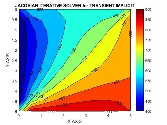
1.JACOBI METHOD	4746	0.7028
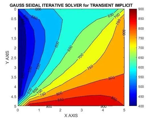
2.GAUSS SEIDAL METHOD	4131	0.4598
3.SOR METHOD	3598	0.1012

THE GRAPH FOR TRANSIENR STATE ITERATIVE METHOD JACOBI METHOD

THE GRAPH FOR TRANSIENR STATE ITERATIVE METHOD GAUSS SEIDAL METHOD

THE GRAPH FOR TRANSIENR STATE ITERATIVE METHOD SUCCESSIVE OVER RELAXATION METHOD

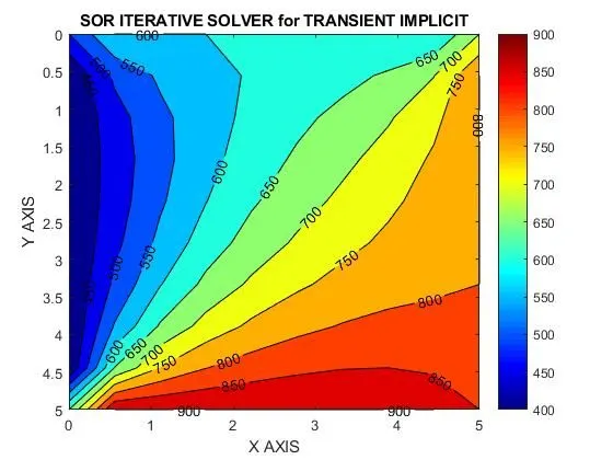
CONCLUSION: HENCE THE CONCLUSION THAT CAN BE DRAWN FROM THE STEADY STATE EQUATIONS AND ITERATIONS IS THAT THE ITERATION IS IN ORDER JACOBI>GAUSS SEIDAL>SOR & THE SWIFTNESS OF EQUATION SOLVING IS IN THE ORDER SOR>GAUSS-SEIDAL>JACOBI. THROUGH THIS CHALLANGE WE HAVE SEEN HOW TO DISCRETIZE AN ELLIPTICAL TIME DEPENDENT EQUATION AND TO SOLVE IT BOTH EXPLICITLY AND IMPLICITLY IN STEADY AND TRANSIENT STATE. THE GRAPHS AND OUTPUTS ARE QUIET PROMICING.THE CODES ARE ATTACHED BELOW IN .m FORMAT ALONG WITH GRAPG JPEG.