Week 1- Mixing Tee
AIM-To set up steady-state simulations to compare the mixing effectiveness when hot inlet temperature is 360C & the Cold inlet is at 190C.
INTRODUCTION:
Ansys Fluent is the industry-leading fluid simulation software known for its advanced physics modeling capabilities and industry leading accuracy.Ansys Fluent gives you more time to innovate and optimize product performance. Trust your simulation results with a software that has been extensively validated across a wide range of applications. With Ansys Fluent, you can create advanced physics models and analyze a variety of fluids phenomena—all in a customizable and intuitive space.
OBJECTIVE:
In this challenge we will be simulating a flow through tee joint where air at 36degree C will mix with air at 19 degree C. We jeve 4 cases for this.
1.Finding out which method k-epsilon or k-omega is better at giving best results.
2.Flow through short pipe at hot air at 3m/s and cold air at 6 m/s.
3.Flow through short pipe at hot air at 3m/s and cold air at 12 m/s.
4.Flow through long pipe at hot air at 3m/s and cold air at 6 m/s.
5.Flow through long pipe at hot air at 3m/s and cold air at 12 m/s.
WE WILL BE PROVIDING THE BELOW RESULT FOR EACH CASE:
- Velocity and temperature contour plots on the cut planes along and across the pipe.
- Velocity and temperature line plots along and across the length of the pipe.
AFTER PERFORMING THE ABOVE EXPERIMENTS WE WILL BE PROVIDING A MESH INDEPENDENT STUDY TO SHOW THE EFFECT OF MESH SIZE ON THE SOLUTION
THEORY:
In a mixing tee a fluid with 2 different temperature are coming through two inlets and is getting mixed inisde a pipe and the effectiveness of mixing is evaluated on parameters like velocity of cold and hot fluid. Also we perform this study to reach optimum cooling and good mixing. Now let us see the general setup of the experiments. Let us see which viscous model shall we use k-epsilon or k_omega.
But first let us knw what k-epsilon and k-omega is.
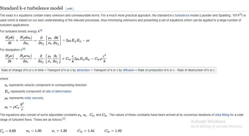
k-epsilon:
K-epsilon (k-ε) turbulence model is the most common model used in CFD to simulate mean flow characteristics for tutbulant flow conditions. It is a two equation model that gives a general description of turbulence by means of two transport equations (PDEs). The original impetus for the K-epsilon model was to improve the mixing-length model, as well as to find an alternative to algebraically prescribing turbulent length scales in moderate to high complexity flows.
- The first transported variable is the turbulent kinetic energy (k).
- The second transported variable is the rate of dissipation of turbulent kinetic energy (ε).
k-omega:
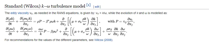
In computational fluid dynamics, the k–omega (k–ω) turbulence model is a common two-equation turbulence model, that is used as an approximation for the Reynolds-averaged Navier–Stokes equations (RANS equations). The model attempts to predict turbulence by two partial differential equations for two variables, k and ω, with the first variable being the turbulence kinetic energy (k) while the second (ω) is the specific rate of dissipation (of the turbulence kinetic energy k into internal thermal energy).
PROCEDURE:
FIRST WE HAVE RUN A TEST BETWEEN KOMEGA NA KEPSILON TO DETERMINE WHICH MODEL TO USE IN ALL THE ABOVE EXPERIMENTS. THE RESULTS ARE AS BELOW.

As a matter of fact we can clearly see that the mixing has reached a lower value when the model is solved by k-epsilon turbulance model under same mesh and other parameter . Kenceforth we will use k-epsilon model to perform our simulations.
Let us discuss why is there such a difference.
The SST k-omega model reduces to a standard k-epsilon model away from walls.
Near walls, the SST k-omega uses the the omega formulation whereas the realizable k-epsilon uses the epsilon formulation.
The two models differ in their approach both near walls and away from walls.
The SST k-omega model is generally thought to be better near walls, but because it reduces to the standard k-epsilon model away from walls and not the realizable k-epsilon model, it also has weaknesses.
The two models are very different and it should be no surprise that significant differences in results can be obtained from each model (this should be considered the norm rather than unusual).
HENCE WE ARE USING THE k-epsilon TURBULANCE MOEL TO SOLVE THIS CHALLENGE.
THE SETUP IS SAME FOR ALL THE 4 SIMULATION EXCEPT THE VELOCITIES AT THE INLET.
SO LET US TAKE A LOOK AT THE COMMONALITIES OF THE SIMULATION STEP BY STEP.
STEP 1: WE ARE PROVIDED WITH A STEP FILE OF MIXING TEE. FIRST WE HAVE TO IMPORT THE GEOMETRY INTOO ASNYS SPACECLAIM.
STEP 2: THEREAFTER WE HAVE TO EXTRACT THE VOLUME OUT OF THE SOLID OBJECT USING THE FOLLOWING TAB.
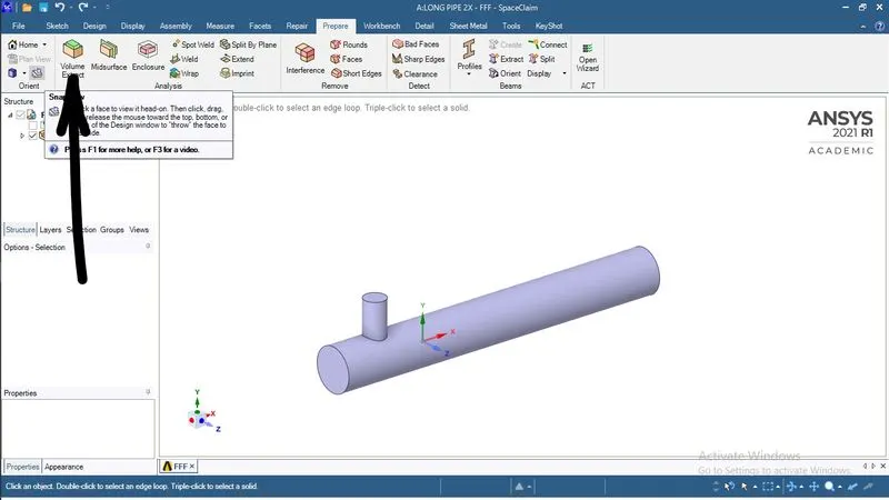
STEP 3: AFTER THIS THE VOUME GETS GENERATED AND WE HAVE TO MANUALLY DISBLE THE PHYSICS OF THE 3D MODEL SO THAT IT IS THE ONLY FLUID DOMAIN THAT TAKES PART IN SIMULATION.
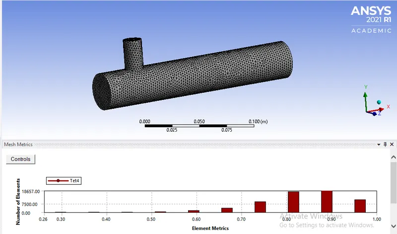
STEP 4: HERE WE CLOSE SPACECLAIN AND OPEN MESHING. WE GIVE HEREA MESH SIZE OF 0.0025 m WHICH IS 2.5 mm AND GENERATE THE MESH.THE MESH LOOKS AS FOLLOWS.
STEP 5: HERE IT INVOLVES GIVING NAMES SELECTION TO INLET AND OUTLET. THE HOT FLUIDE IS COMING IN X DIRECTION AT 3m/S AT 36DEGREE C. THE COLD FLUID IS COMING ALONG Y AXIS AT 6/12m/s AT 19 DEGREE C. THE OUTLET GIVES OUT THE MIXED TEMPERATURE AND VELOCITY OF THE TWO.
THE NAMES SELECTIONS ARE inletx, inlet y, outlet.
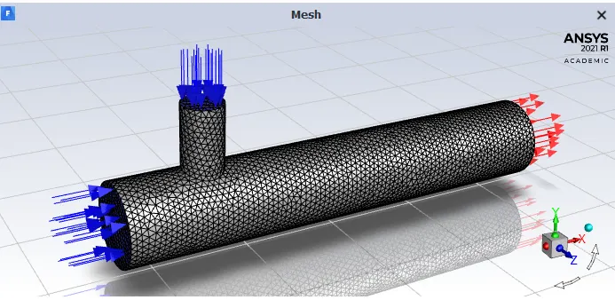
STEP 6: HERE IT INVOLVES OPENNING THE SETUP OR CFX OF THE FLUENT WHERE WE CHOOSE OUR SOLVING TECHNIQUE BY PARALLEL PROCESSOR IF YOUR LISENCE ALLOWS YOU.
STEP 7: HERE WE ASSIGN MATERIAL TO THE VOLUME. IN THIS CASE THE FLUID IS AIR HAVING DENSITY OF 1.229KG/M^3
STEP 8:HERE WE CHOOSE OUR VISCOUS TURBULANT MODEL WHICH IS k-epsilon AND ALSO CHECKMARK THE ENERGY BOX BECAUSE THERMAL HEAT TRANSFER IS GOING TO TAKE PLACE IN THE SYSTEM WHICH REQUIRES ENERGY EQUATION TO BE SOLVED.
STEP 9: IN THIS STEP WE WILL UNCHECK THE DEFAULT CONVERGENCE CRITERIA AT THE RESIDUAL TAB IN SOLUTION.
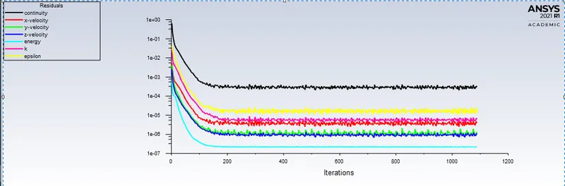
THE SOLUTION IS ASSUEMED TO BE CONVERGED WHEN THE RESIDUAL VALUES REACH A STRAIGHT LINE.
STEP 10: HERE IT INVOLVES DEFINING THE AREA WEIGHTED ABERAGE OF TEMPERATURE AND VELOCITY AT OUTLET BY CREATING PLOTS AND REPORTS. THIS WILL HELP US TO KNOW THE VELOCITY AND TEMPERATURE OF MIXING AT THE OUTLET.
STEP 11:AFTER THE SETUP IS COMPLETE IT IS TIME TO INITIALIZE THE MODEL IN HYBRID MODE.
STEP 12: AFTER INITIALIZING WE GO TO RUN CALCULATION TAB AND AND ENTER OUR DESIRED NUMBER OF ITERATON i.e. 250 AND HIT CALCULATE.
THE SIMULATION WILL RUN AND GIVE US THE CONVERGED RESULT.
STEP 13: AFTER SOLVING TO VISUALIZE THE RESULT WE NEED TO OPEN CFD POST PROCESSING OR RESULTS.
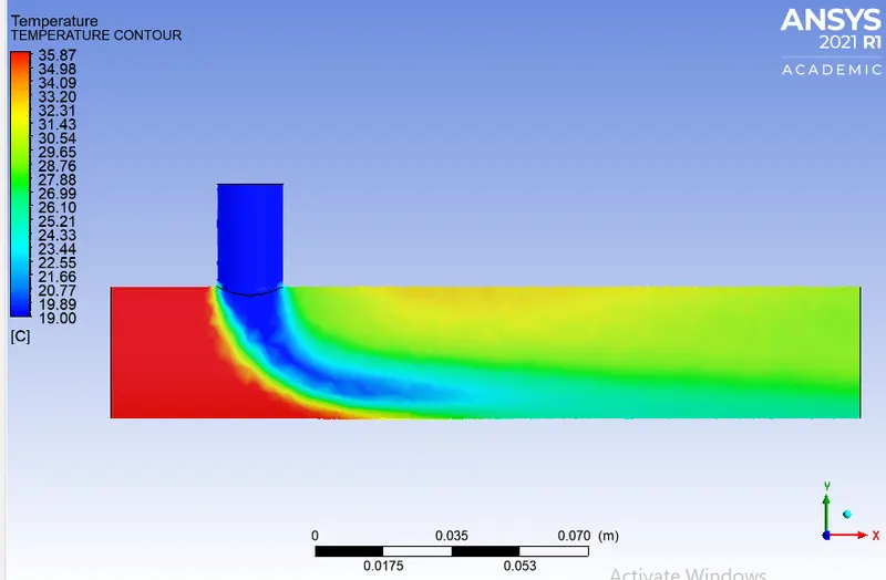
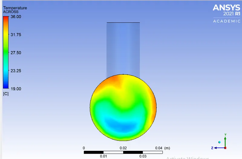
STEP 14: HERE IT INVOLVES CREATING PLANE USING THE LOCATION TOOL TO CREATE TWO PLANES , ONE FOR TEMPERATURE AND ONE FOR VELOCITY IN BOTH XY AND YZ PLANES RESPECTIVELY TO GENERATE THE FLUID PARAMETERS AND GENERATE CONTOUR PLOTS. EXAMPLES FOR TEMPERATUR CONTOUR PLOTS ARE GIVEN BELOW.
TEMP ALONG THE PIPE. TEMP ACROSS THE PIPE.
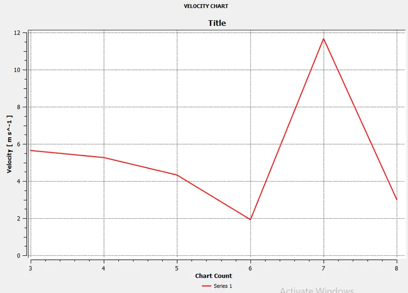
STEP 15:WE ALSO NEED TO THEN CREATE A LINE PROBE FOR TEMPERATURE AND VELOCITY EACH SO THAT WE CAN OBTAIN LINE PLOTS. THE EXAMPLE FOR VELOCITY LINE PLOT IS HERE AS BELOW.
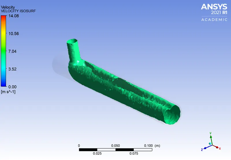
STEP 15: AFTER THESE BASIC STEPS ARE DONE WE CAN VISUALIZE THE VOLUME USING ISOSURFACE TOOL WHICH LOOKS AS BELOW.
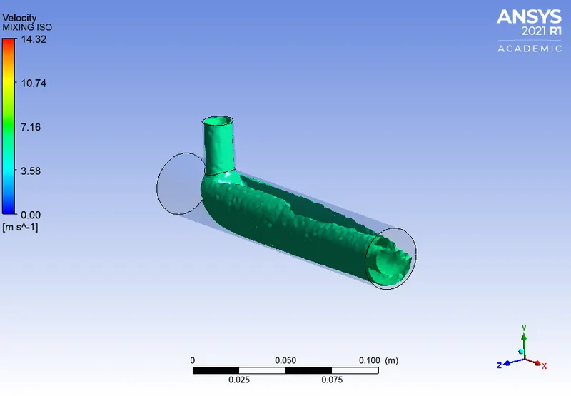
THUS THROUGH ALL THESE STEPS WE CAN SUCCESSFULLY COMPUTE THE SIMULATION.
NOTE:ALL THE ABOVE DISCUSSSION CONCERNS THE COMMON PROCEDURE BETWEEN ALL THE 4 SIMULATION. THE DETAILED OUTLET RESULTS PLOTS AND GRAPHS ARE DISCUSSED FURTHER BELOW.
RESULTS
NOTE : TWO INLET TEMPERATURES ARE SAME FOR ALL THE CASES.
CASE 1:Flow through short pipe at hot air at 3m/s and cold air at 6 m/s.
TEMPERATURE CONTOUR PLOT (ALONG TEE XY PLANE) VELOCITY CONTOUR PLOT(ALONG TEE XY PLANE)
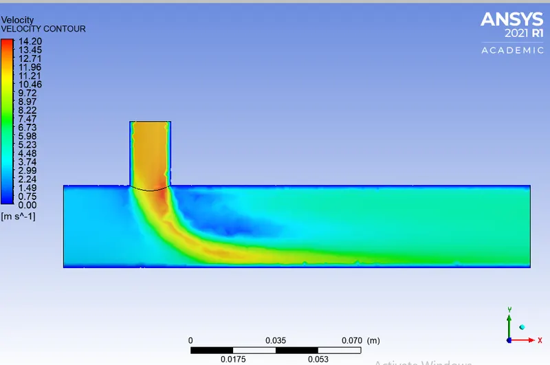
TEMPERATURE CONTOUR PLOT (ACROSS TEE YZ PLANE) VELOCITY CONTOUR PLOT(ACROSS TEE YZ PLANE)
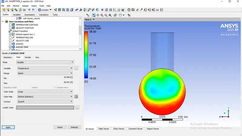
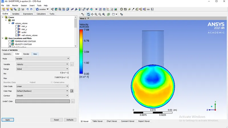
TEMPERATURE LINE PLOT VELOCITY LINE PLOT
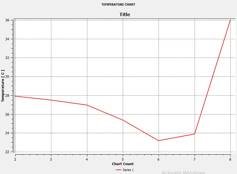
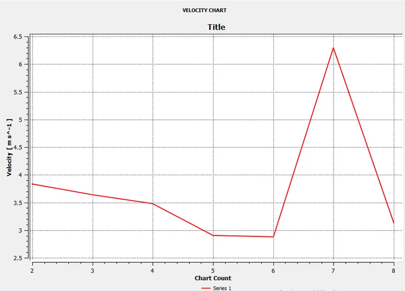
THE NUMBER OF ITERATION TO CONVERGENCE CAN BE SEEN FROM THE BELOW RESIDUAL GRAPH WHICH IS 290 ITRATIONS TO BECOMING FLAT.
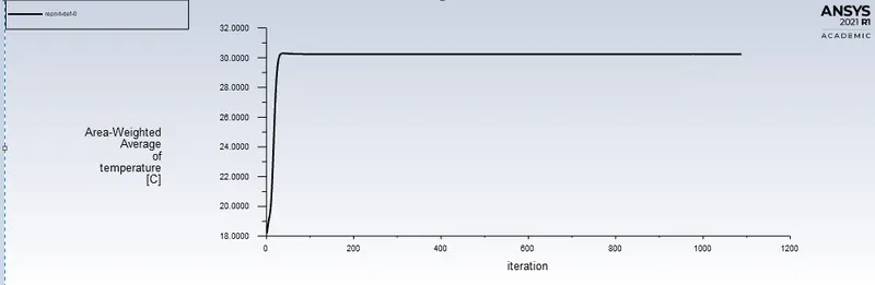
ALSO AFTER CONVERGENCE THE OUTLET TEMPERATURE ALSO BECOMES CONSTANT AS DEPICTED BY THE AREA WEIGHTED AVERAGE GRAPH.
THE RESULTS FOR THE ABOVE CASE ARE AS FOLLOWS:

THESE ARE THE OBSERVATIONS OF THE FIRST SIMULATION.
CASE 2: Flow through short pipe at hot air at 3m/s and cold air at 12 m/s.
TEMPERATURE CONTOUR PLOT (ALONG TEE XY PLANE) VELOCITY CONTOUR PLOT(ALONG TEE XY PLANE)
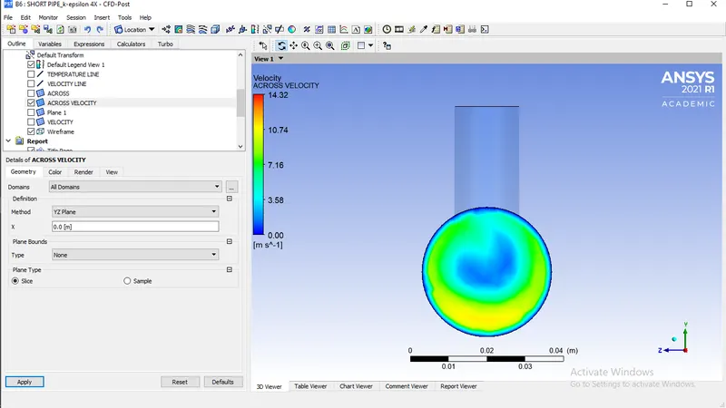
TEMPERATURE CONTOUR PLOT (ACROSS TEE YZ PLANE) VELOCITY CONTOUR PLOT(ACROSS TEE YZ PLANE)
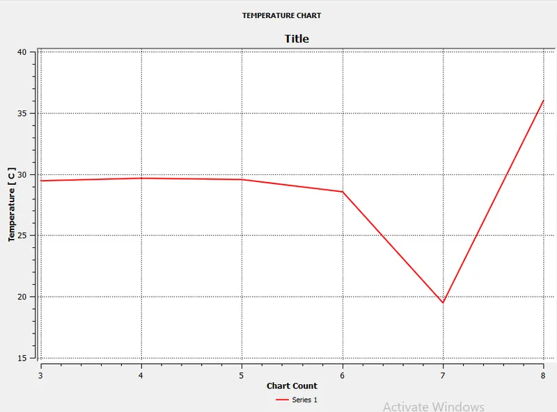
TEMPERATURE LINE PLOT VELOCITY LINE PLOT
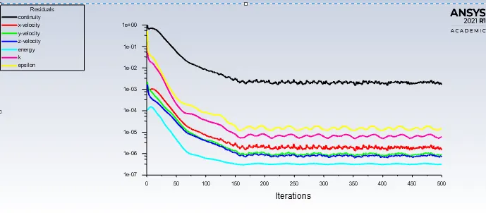
THE NUMBER OF ITERATION TO CONVERGENCE CAN BE SEEN FROM THE BELOW RESIDUAL GRAPH WHICH IS 290 ITRATIONS TO BECOMING FLAT.
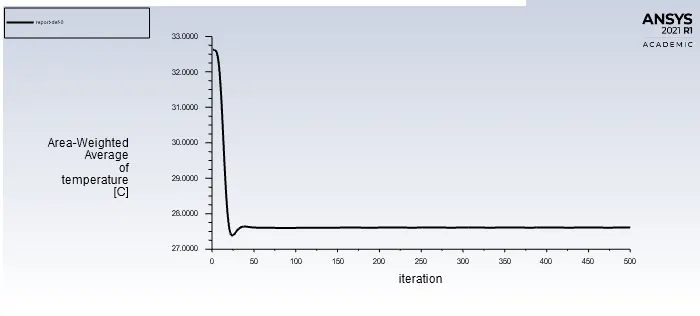
ALSO AFTER CONVERGENCE THE OUTLET TEMPERATURE ALSO BECOMES CONSTANT AS DEPICTED BY THE AREA WEIGHTED AVERAGE GRAPH.
HERE WE ARE TRYING TO VISUALIZE THE 3D FLOW OF THE MIXING USING THE 3D VIEWER TOOL IN ANSYS FLUENT POST.
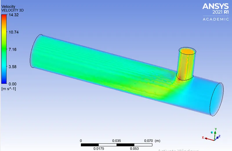
THE RESULTS FOR THE ABOVE CASE ARE AS FOLLOWS:

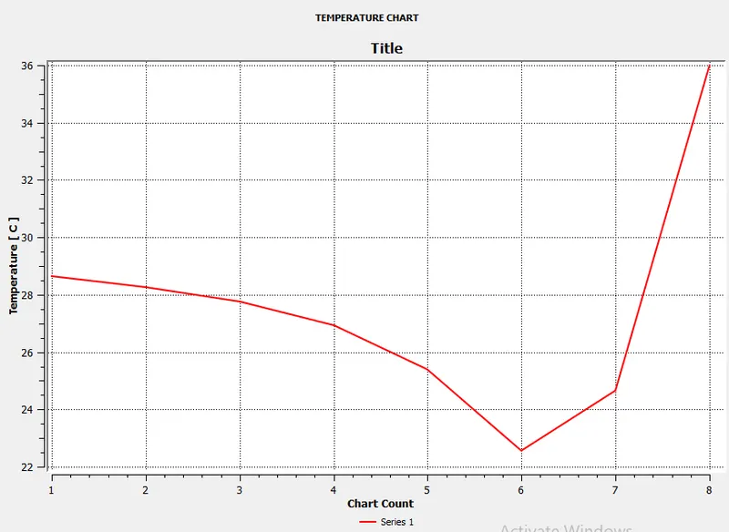
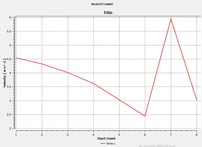
CASE 3: Flow through LONG pipe at hot air at 3m/s and cold air at 6 m/s.
TEMPERATURE CONTOUR PLOT (ALONG TEE XY PLANE) VELOCITY CONTOUR PLOT(ALONG TEE XY PLANE)
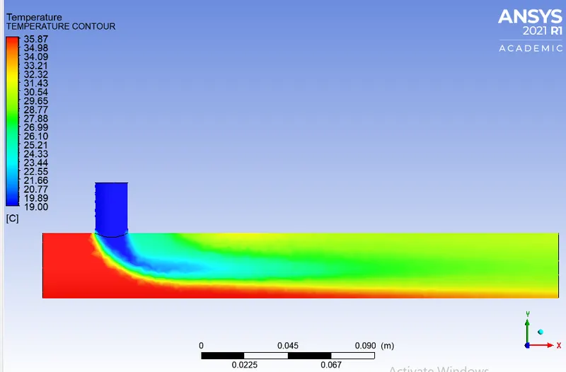
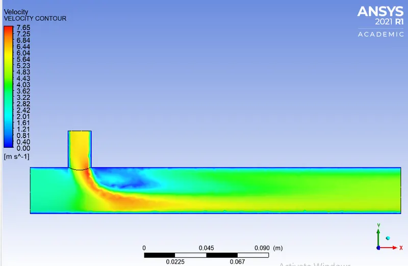
TEMPERATURE CONTOUR PLOT (ACROSS TEE YZ PLANE) VELOCITY CONTOUR PLOT(ACROSS TEE YZ PLANE)
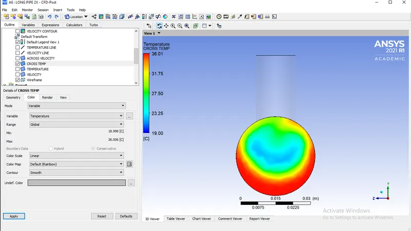
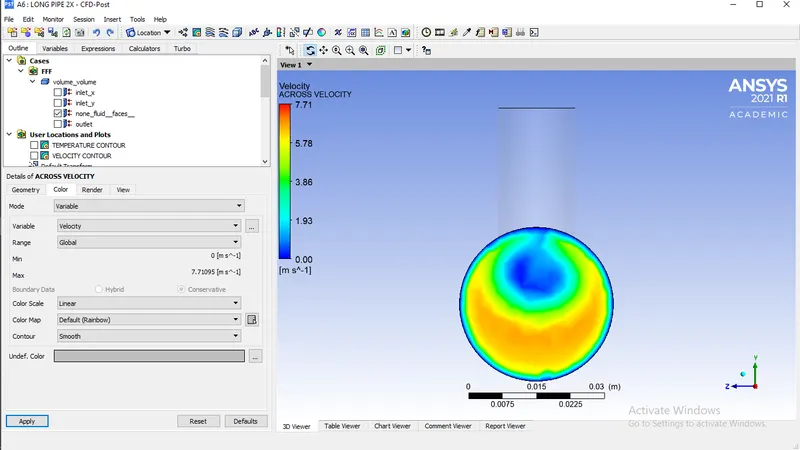
TEMPERATURE LINE PLOT VELOCITY LINE PLOT
THE NUMBER OF ITERATION TO CONVERGENCE CAN BE SEEN FROM THE BELOW RESIDUAL GRAPH WHICH IS 290 ITRATIONS TO BECOMING FLAT.
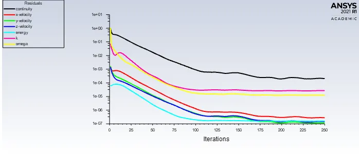
ALSO AFTER CONVERGENCE THE OUTLET TEMPERATURE ALSO BECOMES CONSTANT AS DEPICTED BY THE AREA WEIGHTED AVERAGE GRAPH.
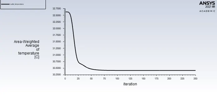
THE RESULTS FOR THE ABOVE CASE ARE AS FOLLOWS:

CASE 4: Flow through LONG pipe at hot air at 3m/s and cold air at 12 m/s.
TEMPERATURE CONTOUR PLOT (ALONG TEE XY PLANE) VELOCITY CONTOUR PLOT(ALONG TEE XY PLANE)
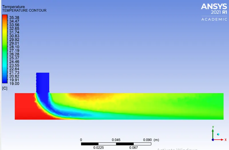
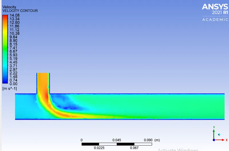
TEMPERATURE CONTOUR PLOT (ACROSS TEE YZ PLANE) VELOCITY CONTOUR PLOT(ACROSS TEE YZ PLANE)
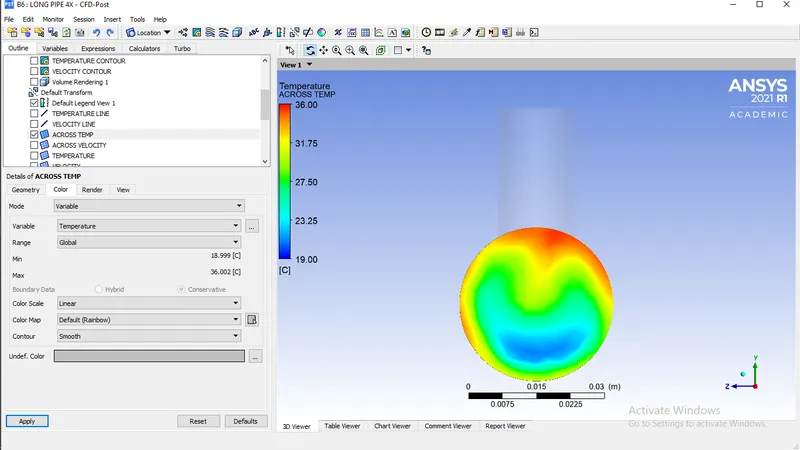
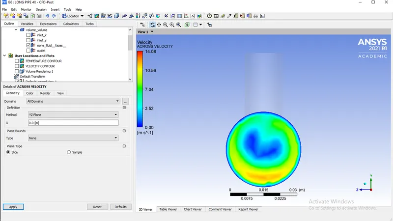
TEMPERATURE LINE PLOT VELOCITY LINE PLOT
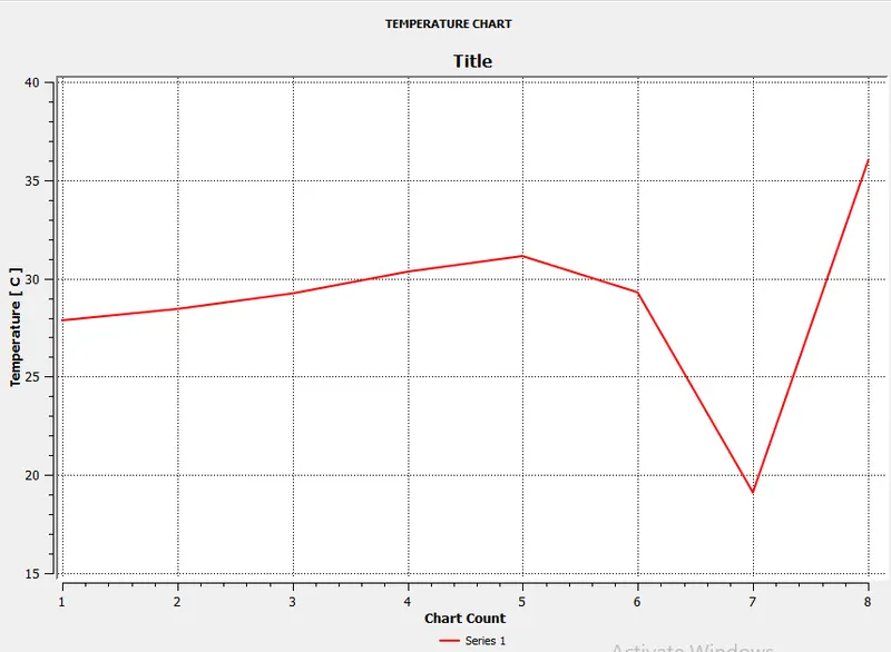
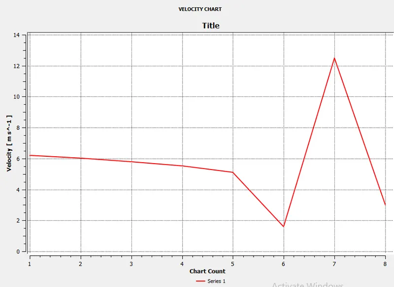
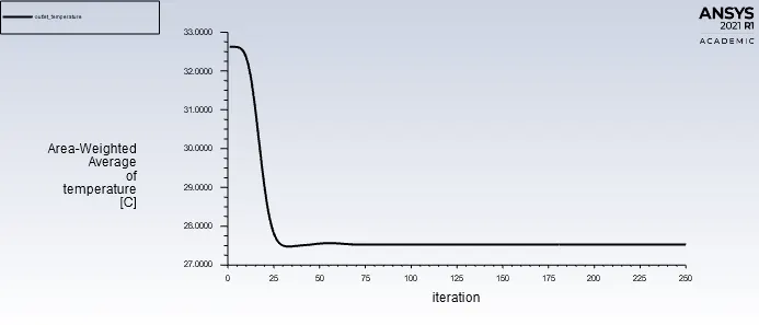
THE NUMBER OF ITERATION TO CONVERGENCE CAN BE SEEN FROM THE BELOW RESIDUAL GRAPH WHICH IS 290 ITRATIONS TO BECOMING FLAT.
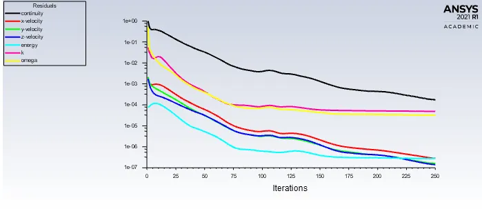
ALSO AFTER CONVERGENCE THE OUTLET TEMPERATURE ALSO BECOMES CONSTANT AS DEPICTED BY THE AREA WEIGHTED AVERAGE GRAPH.
HERE WE ARE TRYING TO VISUALIZE THE 3D FLOW OF THE MIXING USING THE 3D VIEWER TOOL IN ANSYS FLUENT POST.
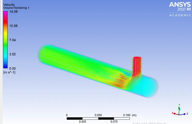
THE RESULTS FOR THE ABOVE CASE ARE AS FOLLOWS:

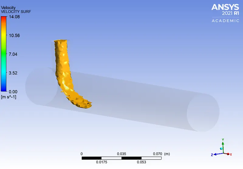
LET US TAKE A LOOK AT THE DIFFERENT STEPS OF FLUID FLOW AT 3m/s 12m/s AND MIXING VELOCITY.
3M/S INLET
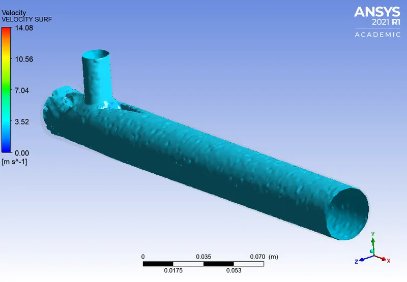
12M/S INLET
OUTLET MIXING 5.999M/S
MESH INDIPENDENT ANALYSIS.
WE HAVE RUN A MESH INDIPENDENT ANALYSIS FOR LONG TEE WITH MOMENTUM RATIO OF 4.
THE DIFFERENCE IS LISTED BELOW.

THE GREATER THE LENGTH OF PIPE RESULTS IN BETTER MIXING.
HIGER THE MOMENTUM RATIO BETTER IS THE VOLUME FLOW RATE HENCE GREATER AMOUNT OF COLD AIR GETS MIXED WITH THE HOT FLUID TO ACHIEVE EFFECTIVE COOLING.
CONCLUSION:
HENCE FROM THIS CHALLENGE WE HAVE LEARNT THE FOLLOWING
1.LONGER LENGTH OF PIPE INCREASES EFFECTIVENESS OF MIXING.
2.GREATER MOMENTUM RATIO OF COLD AIR ACHIEVES EFFECTIVE COOLING.
3.MESH SIZE IS IMPORTENT FOR GENERATING ACCURATE RESULT.
4.WE HAVE SEEN VARIOUS METHODS TO VISUALIZE THE TEMPERATURE AND VELOCITY CHANGE THROUGH THE TEE AND AT OUTLET.
PLEASE FIND HERE ATTACHED THE RAR FILE FOR FURTHER DOCUMENTS AND ANSYS FILES.
THANK YOU.