Week 3.5 - Deriving 4th order approximation of a 2nd order derivative using Taylor Table method
PLEASE NOTE ALL THE PROGRAMS ARE SUFFICIENTLY LOADED WITH COMMENTS TO UNDERSTAND THE CODE BETTER!!!!!
AIM:-
Deriving 4th order approximation of a 2nd order derivative using Taylor Table method.
THEORY:-
DISCERETIZATION IS ONE OF THE MOST IMPORTENT STEP IN COMPUTING DIFFICULT GRID PROBLEMS.SO IN THIS CHALLENGE WE WOULD BE DEALING WITH HOW TO DERIVE 4TH ORDER APPROXIMATION USING TAYLORS TABLE METHOD. LATER USING THE DERIVED EQUATION WE WILL BE MOVING TOWARDS THE SOLVING OF A FUNCTION exp(x)cos(x).WE WOULD BE PRODUCING BOTH ANALYTICAL AND APPROXIMATION AND COMPARE THE ERROR DIFFERENCE OF LEFT SKEWD,RIGHT SKEWED AND CENTRAL 4TH ORDER APPROXIMATION.
SUPPLIED INFORMATIONS:-
f(x)=exp(x)*cos(x)
ASSUMED INFORMATIONS:-
x=pi/3
dx=20equispaced values between pi/40 and pi/4
PROCEDURE:-
FIRSTLY BEFORE MOVING ON WITH THE PROGRAMMING COME LET US SEE HOW CAN WE DERIVE THE 4TH ORDER APPROXIMATION FOR CENTRAL,RIGHT SKEWED AND LEFT SKEWED APPROXIMATION.
LEFT SKEWED IS A CONCEPT WHERE WE CONSIDER POINTS ONLY ON THE LEFT SIDE OF A PARTICULAR GRID POINT.
RIGHT SKEWED IS A CONCEPT WHERE WE CONSIDER POINTS ONLY ON THE RIGHT SIDE OF A PARTICULAR GRID POINT.
CENTRAL DIFFERENCE METHOD IS THE PROCESS BY WHICH WE TAKE POINTS AND DATA FROM BOTH SIDE OF THE GRID POINT,BOTH POSITIVE AND NEGETIVE.
NOW THE POSSIBLE QUESTION ARISES THAT WHY DO WE NEED 3 TYPES OF 4TH ORDER APPROXIMATION ?
THE ANSWER IS VERY SIMPLE. EVERYTHING DEPENDS ON WHICH APPROXIMATION GIVES THE LEAST ERROR.
ON OTHER HAND ANOTHER REASON IS THAT WHILE SOLVING EQUATION ON BOUNDARY WE WILL HAVE ONLY POINTS ON ANY ONE SIDE EITHER LEFT OR RIGHT. SO THESE ARE THE MAIN REASON WE EXPLORE THESE MANY TYPES OF APPROXIMATION TO REDUCE THE CHANCES OF ERROR AND TO ATTAIN GREATER STABILITY OF OUR RESULT.
LET US GET STARTED WITH THE DERIVATION OF CENTRAL ORDER APPROXIMATION
- FIRST WE WILL START WITH THE 2ND DERIVATIVE 4TH ORDER APPROXIMATION USING CENTRAL DIFFERENCE METHOD.THE DETAILED DERIVATION IS ATTACHED BELOW TO REFER WITH THAT IN THE PROGRAMMING.
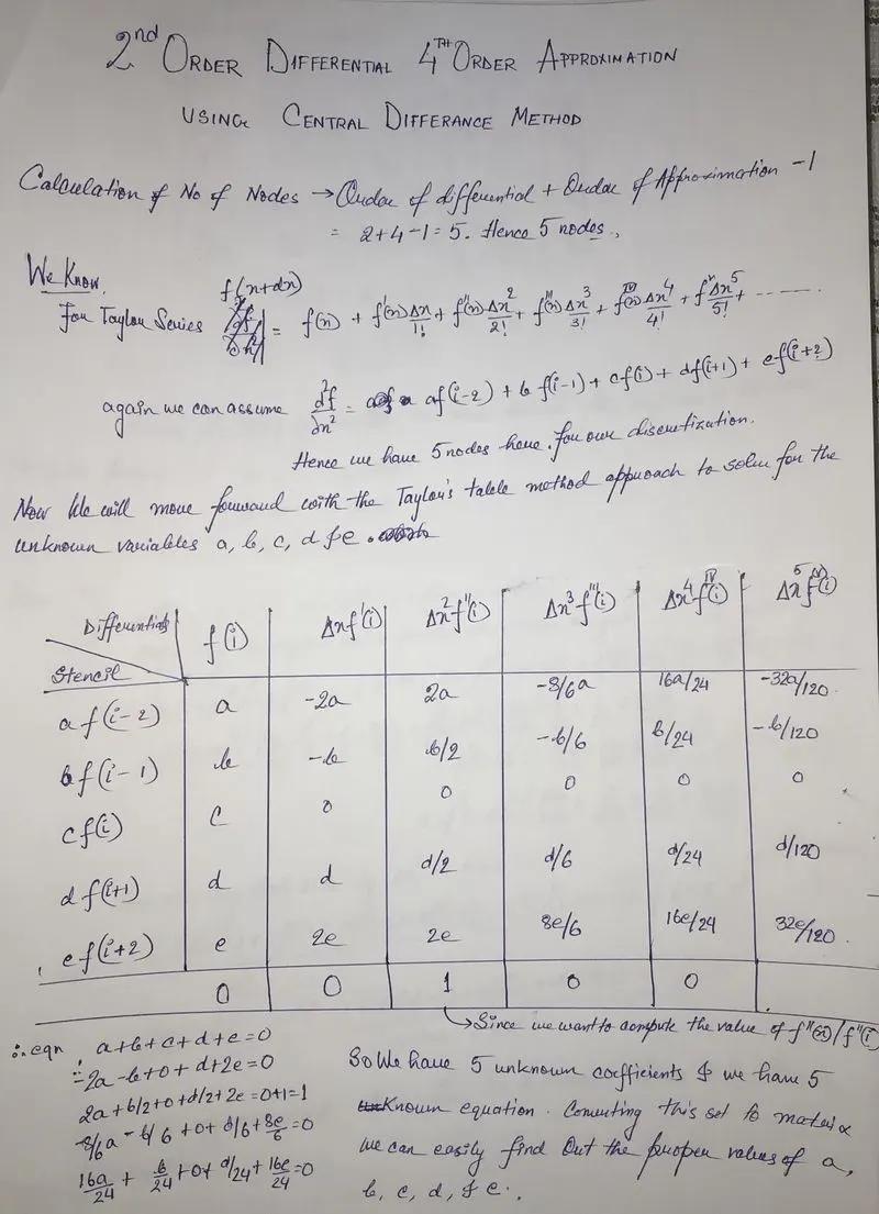
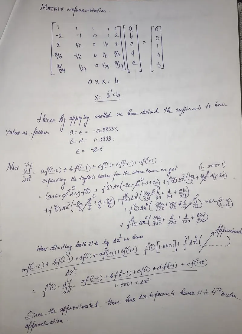
SINCE WE HAVE NOW DERIVED THE EQUATION FOR 4TH ORDER APPROXIMATION WE CAN NOW USE IT IN A CODE TO WRITE A FUNCTION IN MATLAB TO COMPUTE THE ERROR WRT TO ANALYTICAL SOLUTION.
THE ANALYTICAL_SOLUTION IS =-2*exp(x)*sin(x).
NOW WE HAVE OUR RESULT THROUGH CENTRAL DIFFERENCE IN 4TH ORDER APPROXIMATION,WHICH IS fourth_order_approx=((a*exp(x-(2*dx))*cos(x-(2*dx)))+(b*exp(x-dx)*cos(x-dx))+(c*exp(x)*cos(x))+(d*exp(x+dx)*cos(x+dx))+(e*exp(x+(2*dx))*cos(x+(2*dx))))/(dx*dx*1.0001)
THEREFORE THE ABSOLUTE ERROR WILL BE =IANALYTICAL_SOLUTION-fourth_order_approxI
LET US NOW REPRESENT THIS IN PROGRAM AS FOLLOWING:-BY CREATING THIS WE ARE DEVELOPING THE STEPPING STONES OF THE MAIN PROGRAM.
function [siera]=fourth_central(x,dx)

%actual_function=(e^x)*sin(x)

a=-0.0833;
b=1.3333;
c=-2.5;
d=1.3333;
e=-0.0833;

analytical_solution=-2*exp(x)*sin(x);
fourth_order_approx=((a*exp(x-(2*dx))*cos(x-(2*dx)))+(b*exp(x-dx)*cos(x-dx))+(c*exp(x)*cos(x))+(d*exp(x+dx)*cos(x+dx))+(e*exp(x+(2*dx))*cos(x+(2*dx))))/(dx*dx*1.0001)

siera=abs(analytical_solution-fourth_order_approx)

end
YOU MUST WONDER HOW THE a,b,c,d,e VALUES WE GOT. WELL IF YOU TAKE A LOOK IN THE DERIVATION YOU WILL SEE TWO MATRICES MULTIPLIED TO GIVE A 5X1 MATRIX.SO WE USE THE INVERSE OF 5X5 MATRIX AND MULTIPLY WITH 5X1 TO RECEIVE A 5/1 MATRIX WHICH GIVES US THE FOLLOWING DATA.THE CODE IS ATTACHED BELOW AS CODE c.m
j=[1 1 1 1 1
    -2 -1 0 1 2
    2 .5 0 .5 2
    -8/6 -1/6 0 1/6 8/6
    16/24 1/24 0 1/24 16/24]
k=[0;0;1;0;0]
x=(j^(-1))*k
a=x(1)
b=x(2)
c=x(3)
d=x(4)
e=x(5)
- NOW LET US TAKE A LOOK IN THE RIGHT SKEWED APPROXIMATION.
- FIRST WE WILL START WITH THE 2ND DERIVATIVE 4TH ORDER APPROXIMATION USING RIGHT SKEWED METHOD.THE DETAILED DERIVATION IS ATTACHED BELOW TO REFER WITH THAT IN THE PROGRAMMING.
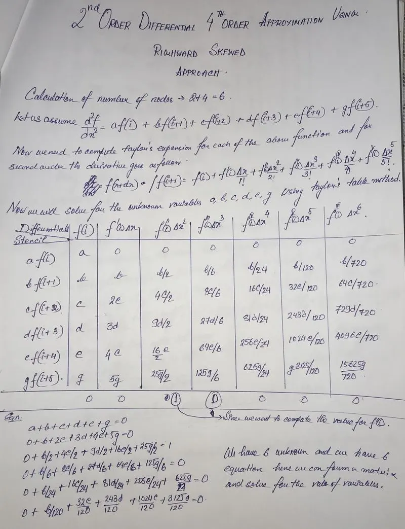
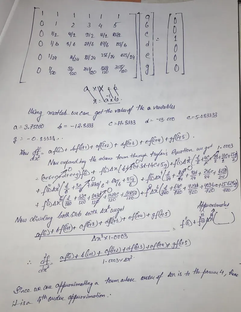
SINCE WE HAVE NOW DERIVED THE EQUATION FOR 4TH ORDER APPROXIMATION WE CAN NOW USE IT IN A CODE TO WRITE A FUNCTION IN MATLAB TO COMPUTE THE ERROR WRT TO ANALYTICAL SOLUTION.
THE ANALYTICAL_SOLUTION IS =-2*exp(x)*sin(x).
NOW WE HAVE OUR RESULT THROUGH SKEWED RIGHT IN 4TH ORDER APPROXIMATION,WHICH IS fourth_order_approx=((a*exp(x)*cos(x))+(b*exp(x+dx)*cos(x+dx))+(c*exp(x+(2*dx))*cos(x+(2*dx)))+(d*exp(x+(3*dx))*cos(x+(3*dx)))+(e*exp(x+(4*dx))*cos(x+(4*dx)))+(g*exp(x+(5*dx))*cos(x+(5*dx))))/(dx*dx*1.0003)
THEREFORE THE ABSOLUTE ERROR WILL BE =IANALYTICAL_SOLUTION-fourth_order_approxI
LET US NOW REPRESENT THIS IN PROGRAM AS FOLLOWING:-BY CREATING THIS WE ARE DEVELOPING THE STEPPING STONES OF THE MAIN PROGRAM.
function[kayotu]=skewed_right(x,dx)

%actual_function=(e^x)*sin(x)

a=3.750000;
b=-12.8333;
c=17.8333;
d=-13;
e=5.08333;
g=-0.8333;
analytical_solution=-2*exp(x)*sin(x);
fourth_order_approx=((a*exp(x)*cos(x))+(b*exp(x+dx)*cos(x+dx))+(c*exp(x+(2*dx))*cos(x+(2*dx)))+(d*exp(x+(3*dx))*cos(x+(3*dx)))+(e*exp(x+(4*dx))*cos(x+(4*dx)))+(g*exp(x+(5*dx))*cos(x+(5*dx))))/(dx*dx*1.0003)

kayotu=abs(analytical_solution-fourth_order_approx)
end
YOU MUST WONDER HOW THE a,b,c,d,e VALUES WE GOT. WELL IF YOU TAKE A LOOK IN THE DERIVATION YOU WILL SEE TWO MATRICES MULTIPLIED TO GIVE A 5X1 MATRIX.SO WE USE THE INVERSE OF 5X5 MATRIX AND MULTIPLY WITH 5X1 TO RECEIVE A 5/1 MATRIX WHICH GIVES US THE FOLLOWING DATA.THE CODE IS ATTACHED BELOW AS CODE dd.m
j=[1 1 1 1 1 1
    0 1 2 3 4 5
    0 1/2 4/2 9/2 16/2 25/2
    0 1/6 8/6 27/6 64/6 125/6
    0 1/24 16/24 81/24 256/24 625/24
    0 1/120 32/120 243/120 1024/120 3125/120]
k=[0;0;1;0;0;0]
x=(j^(-1))*k
a=x(1)
b=x(2)
c=x(3)
d=x(4)
e=x(5)
g=x(6)
- NOW LET US TAKE A LOOK IN THE LEFT SKEWED APPROXIMATION.
- LAST BUT NOT THE LEAST WE WILL START WITH THE 2ND DERIVATIVE 4TH ORDER APPROXIMATION USING LEFT SKEWED METHOD.THE DETAILED DERIVATION IS ATTACHED BELOW TO REFER WITH THAT IN THE PROGRAMMING.
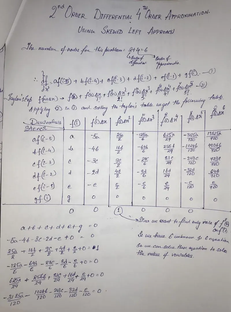
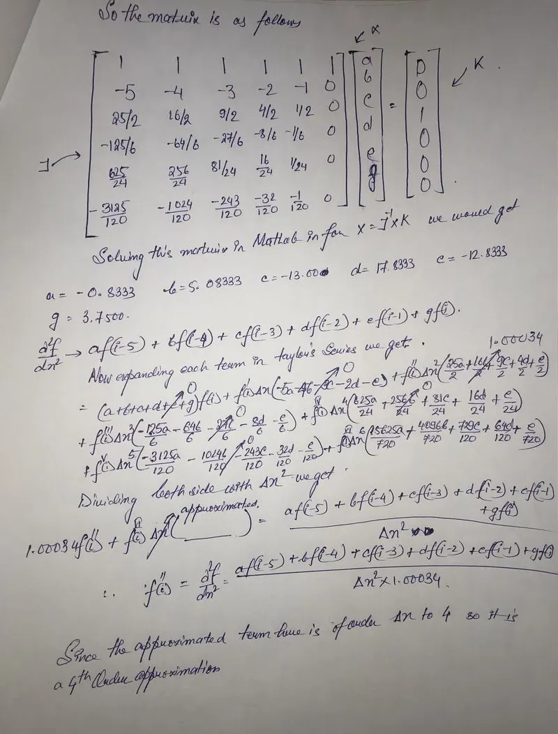
INCE WE HAVE NOW DERIVED THE EQUATION FOR 4TH ORDER APPROXIMATION WE CAN NOW USE IT IN A CODE TO WRITE A FUNCTION IN MATLAB TO COMPUTE THE ERROR WRT TO ANALYTICAL SOLUTION.
THE ANALYTICAL_SOLUTION IS =-2*exp(x)*sin(x).
NOW WE HAVE OUR RESULT THROUGH SKEWED LEFT IN 4TH ORDER APPROXIMATION,WHICH IS fourth_order_approximation=((a*exp(x-(5*dx))*cos(x-(5*dx)))+(b*exp(x-(4*dx))*cos(x-(4*dx)))+(c*exp(x-(3*dx))*cos(x-(3*dx)))+(d*exp(x-(2*dx))*cos(x-(2*dx)))+(e*exp(x-dx)*cos(x-dx))+(g*exp(x)*cos(x)))/(1.0003*dx*dx)
THEREFORE THE ABSOLUTE ERROR WILL BE =IANALYTICAL_SOLUTION-fourth_order_approxI
LET US NOW REPRESENT THIS IN PROGRAM AS FOLLOWING:-BY CREATING THIS WE ARE DEVELOPING THE STEPPING STONES OF THE MAIN PROGRAM.
function [montana]=skewed_left(x,dx)

%actual_function=exp(x)*sin(x)
a=-0.8333;
b=5.08333;
c=-13;
d=17.8333;
e=-12.8333;
g=3.75;
analytical_solution=-2*exp(x)*sin(x);
fourth_order_approximation=((a*exp(x-(5*dx))*cos(x-(5*dx)))+(b*exp(x-(4*dx))*cos(x-(4*dx)))+(c*exp(x-(3*dx))*cos(x-(3*dx)))+(d*exp(x-(2*dx))*cos(x-(2*dx)))+(e*exp(x-dx)*cos(x-dx))+(g*exp(x)*cos(x)))/(1.0003*dx*dx)

montana=abs(analytical_solution-fourth_order_approximation)


end
YOU MUST WONDER HOW THE a,b,c,d,e VALUES WE GOT. WELL IF YOU TAKE A LOOK IN THE DERIVATION YOU WILL SEE TWO MATRICES MULTIPLIED TO GIVE A 5X1 MATRIX.SO WE USE THE INVERSE OF 5X5 MATRIX AND MULTIPLY WITH 5X1 TO RECEIVE A 5/1 MATRIX WHICH GIVES US THE FOLLOWING DATA.THE CODE IS ATTACHED BELOW AS CODE ee.m
j=[1 1 1 1 1 1
    -5 -4 -3 -2 -1 0
    25/2 16/2 9/2 4/2 1/2 0
    -125/6 -64/6 -27/6 -8/6 -1/6 0
    625/24 256/24 81/24 16/24 1/24 0
    -3125/120 -1024/120 -243/120 -32/120 -1/120 0]
k=[0;0;1;0;0;0]
x=(j^(-1))*k
a=x(1)
b=x(2)
c=x(3)
d=x(4)
e=x(5)
g=x(6)
SO NOW WE HAVE SET UP THE STAGE TO GO AHEAD WITH THE MAIN PROGRAM WHICH WILL CALCULATE THE ERROR FOR 20 DIFFERENT VALUES OF dx RANGING FROM pi/40 TO pi/4.
WE NOW HAVE A READY FUNCTION TO BE USED IN OUT MAIN PROGRAM TO COMPUTE THE ERROR TERMS.
BUT WE NEED TO KEEP IN MIND THAT WE NEED TO COMPUTE THE ERROR FOR 20 DIFFERENT VALUES OF dx.SO WE NEED A FOR LOOP TO EXECUTE THE 20 APPROXIMATION FOR EACH METHOD AND TO STORE THE VALUES IN A PARTICULAR VARIABLE.
HERE IS HOW WE DO IT.
- FIRST WE INPUT THE STEP COUNTER FOR THE FOR LOOP.THE LOOP IS STARTING FROM 1 AND CONTINUING TILL LENGTH OF (dx) WHICH IS 20. SO THE LOOP WILL REPEAT ITSELF FOR 20 TIMES.
- DURING EACH LOOP IT WILL EXECUTE ALL THE FUCTIONS DEFINED INSIDE THE LOOP. SO LET US TAKE A LOOK AT WHAT WE DEFINE INSIDE THE FOR LOOP.
- THE SYNTAX USED IN THE LOOP IS SHOWN BELOW
- for i=1:length(dx); %here we are determining the length or the size of i . Size of i determines the number of times by which the loop will repeat itself.The step is 20 times as there are 20 values of dx.
- error_right(i)=skewed_right(x,dx(i))
- refer to the function program to understand the code
Error_right(i) is used so that the variable is converted into an array having 20 values in a row having 20 columns. dx(i) is used to identify which term of the array dx does the program executes during a particular loop.ie for 2nd loop running the value od dx will be equal to the 2nd value in the array of dx.
% same steps are followed for the next two lines ie 26&27
error_left(i)=skewed_left(x,dx(i))
error_central(i)=fourth_central(x,dx(i))
- NOW AFTER THE EXECUTION FOR FOR LOOP WE HAVE THREE SET OF ARRAY NAMELY error_central,error_right,error_left.Each of these contains 20values.
- Now we will proceed with the loglog garph plotting relation between error terms and dx.
- SYNTX GOES AS FOLLOWS:
figure(1)
loglog(dx,error_right)%here we are plotting the loglog graph so that the areas of the precision are closely visible to distinguish
hold on %hold on is used to fit mutiple graph in a single figure window.
loglog(dx,error_left)%similarly the left and central 4th order error terms are plotted below.
loglog(dx,error_central)
%out of the three curves the central fourth order approximation gives the least
%amount of error as it is more closer to the higher negetive order of 10
THE WHOLE PROGRAM IS ATTACHED BELOW FOR FURTHER REFERENCE.THE PROGRAM IS ATTACHED WITH COMMENTS TO UNDERSTAND BETTER.
clear all
close all
clc
%here we are determining the point where we need to compute the function sin(x)/x^3
%we will compute the function t the point x=pi/3
%dx is the small delta steps by which we will discretize the problem  over
%a given range.
x=pi/3;
dx=linspace(pi/40,pi/4,20);%here we are using linspace command to get 20 equispaced values between pi/4 and pi/40
analytical_solution=-2*exp(x)*sin(x);
%previously we have created 3 function indipendently to compute the error
 %in the first,second and fourth order approximation.

for i=1:length(dx)%here we are determining the length or the size of i .
     %size of i determines the number of times by which the loop will
     %repeat itself.the step is 20 times as there are 20 values of dx.

error_right(i)=skewed_right(x,dx(i)) %refer to the function program to understand the code
     %error_right(i) is used so that the variable is converted into
     %an array having 20 values in a row having 20 columns.dx(i) is used to
     %identify which term of the array dx does the program executes during
     %a particular loop.ie for 2nd loop running the value od dx will be
     %equal to the 2nd  value in the array of dx.

    % same steps are followed for the next two lines ie 26&27
error_left(i)=skewed_left(x,dx(i))
error_central(i)=fourth_central(x,dx(i))

end

figure(1)
loglog(dx,error_right)%here we are plotting the loglog graph so that the areas of the  precision are closely visible to distinguish
hold on %hold on is used to fit mutiple graph in a single figure window.
loglog(dx,error_left)%similarly the left and central 4th  order error terms are plotted below.
loglog(dx,error_central)
 %out of the three curves the central fourth order approximation gives the least
   %amount of error as it is more closer to the higher negetive order of 10

grid on
xlabel('dx')
ylabel('CENTRAL,SKEWED RIGHT,SKEWED LEFT ERROR W.R.T ANALYTIC SOLUTION')
 legend('RIGHT SKEWED','LEFT SKEWED','CENTRAL ORDER')
THE PLOT THAT WE GET AFTER THE EXECUTION OF THE CODE IS AS FOLLOWS:-
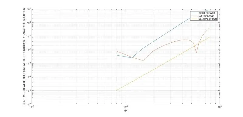
FROM THE ABOVE SET OF POINT IT IS QUITE VISIBLE THAT THE FOURTH ORDER CENTRAL DIFFERENCE GRAPH POINTS ARE GOING FURTHEST TOWARDS THE MINIMUM DIRECTION AND HAVE THE LEAST VALUES.
IMPORTENT INTERPRITATION FROM THE GRAPH:-
- FIRST OF ALL WE CAN VISUALLY SEE THAT THE ERROR TERMS BETWEEN SKEWED LEFT AND SKEWED RIGHT ARE NOT ANY MAJOR.BUT THESE TWO HAVE MUCH GREATER DEGREE OF ERROR WRT CENTRAL DIFFERENCE 4TH ORDER CURVE.
- SECONDLY WE CAN SEE THAT THE SKEWED LEFT & RIGHT HAVE SOME INCREASE IN ERROR AT THE END OF THE CURVE TOWARDS POSITIVE DIRECTION. THIS IS DUE TO THE FACT THAT SMALLER THE dx VALUE GREATER IS THE DEGREE OF ROUND OFF ERROR INCORPORATED IN THE EQUATION. HUGE NUMBER OF SMALL ERRORS SUM UP TO GIVE AN APPRECIABLE INCREASE IN ERROR.
Q.Why a skewed scheme is useful? What can a skewed scheme do that a CD scheme cannot?
ANS. CLEARLY WE CAN SEE THAT THE ERROR IN SKEWED SET IS GREATER THAN CENTRAL DIFFERENCE SCHEME, SO THE OBVIOUS QUESTION IS WHERE DO WE NEED IT AND WHY.THE ANSWER IS WE NEED IT IN A PROBLEM WHERE WE ARE CALCULATING EQUATION ON A BOUNDARY CONDITION.IN SUCH A CASE THERE IS EITHER VALUE ON LEFT OR ON THE RIGHT DEPENDING UPON THE FLOW OF INFORMATION. SO WE CANNOT COMPUTE CENTRAL DIFFERENCING IF WE DONOT GET NEIGHBOURING POINTS BOTH FROM POSITIVE AND NEGETIVE SIDE OF THE GRID. THIS IS WHERE THE NUMERICAL STENCIL OF THE SKEWED SCHEME HELPS TO MINIMIZE THE ERROR AND COMPUTES THE VALUE OF A POINT BY TAKING DATA FROM AND ANY ONE DIRECTION.
CONCLUSION:-
IN THIS CAHALLENGE WE HAVE SUCCESSFULLY COMPUTED THE DERIVATION MANUALLY AND FOUND OUT THE EQUATION FOR SECOND ORDER 4TH ORDER APPROXIMATION FOR CENTRALDIFF,SKEWED RIGHT & SKEWED LEFT ARRANGEMENT.ALSO WE HAVE USED THESE EQUATIONS TO SOLVE A FUNCTION AND CALCULATE ABSOLUTE ERROR W.R.T ANALYTICAL SOLUTION. IT HAVE BEEN FOUND THAT THE ERROR VARIES AS FOLLOWS:-CENTRAL_DIFFERENCE<(SKEWED LEFT/RIGHT).