Week 7 - Simulation of a 1D Super-sonic nozzle flow simulation using Macormack Method
THE CODE IS ATTACHED WELL WITH COMMENTS FOR BETTER UNDERSTANDING.
THE RAR FILE CONTAINING THE RESULTS AND OTHER CODES AND FUNCTIONS ARE ATTACHED WITH THIS PROJECT
AIM
Simulation of a 1D Super-sonic nozzle flow simulation using Macormack Method
OBJECTIVE
In this challenge we are going to simulate the isentropic flow through a quasi 1D subsonic-supersonic nozzle. We will derive both the conservation and non-conservation forms of the governing equations and sovle them using the MacCormack's technique. We need to determine the steady-state temperature distribution for the flow-field variables and investigate the difference between the two forms of governing equations by comparing their solutions.
We need to show the following plots inside your report
1. Steady-state distribution of primitive variables inside the nozzle
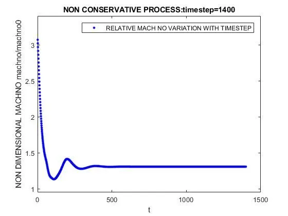
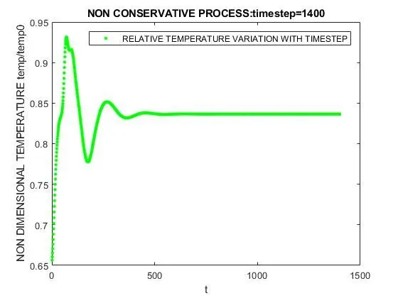
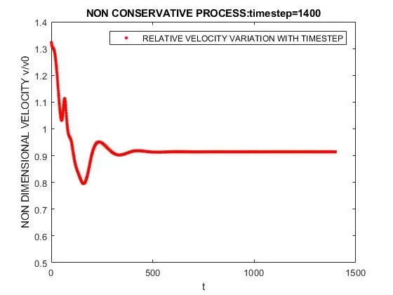
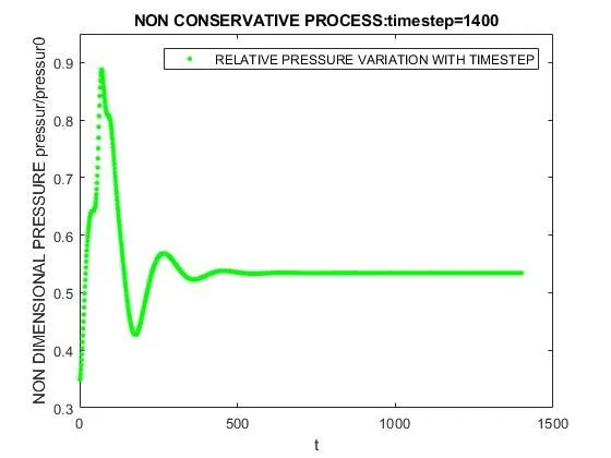
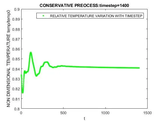
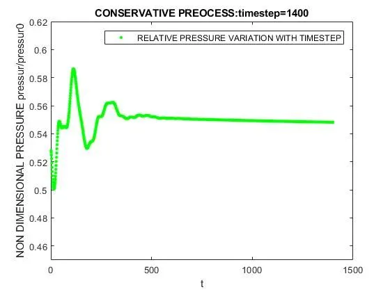
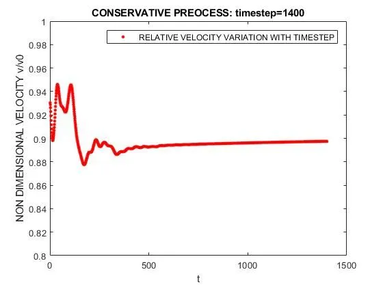
2. Time-wise variation of the primitive variables
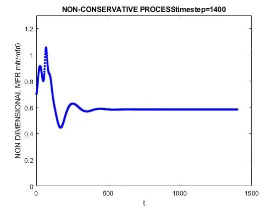
3. Variation of Mass flow rate distribution inside the nozzle at different time steps during the time-marching process
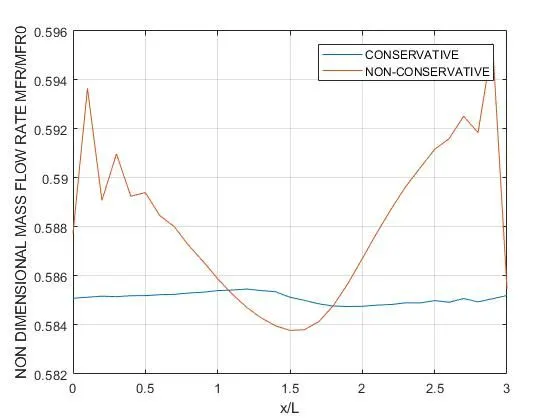
4. Comparison of Normalized mass flow rate distributions of both forms
PROCEDURE
1. Physical description of the flow. The physical aspects of the flow will be described, and pertinent equations and relahonships obtained from the anallytical solution will be reviewed. If experimental data are appropriate, they will be discussed. The purpose here is to give you a physical understanding of the flow
field, to be calculated subsequently with our CFD techniques.
2. CFD solution: intermediate steps. A specific CFD technique will be chosen for the numerical solution of the flow problem. The pertinent partial differential equations or the integral form of the equations, as the case may be, most suited for the specific CFD technique as applied to the specific flow problem will be set forth. The solution will be set up, step by step, and the numerical operations will be carried through in detail for the first few steps. Numbers will be given for all stages of the calculation during these intermediate steps so that you can compare them directly with your own calculations. Such matters as the calculations at internal points, at the boundaries, the numerical implementation of boundary conditions, and the determination of step size (if appropriate) will be covered in detail.
3. CFD solution: final results. Tabulations and graphs of the final numerical solution to the flow field will be given. These final results will be compared with the exact analytical (and/or experimental) results, and an evaluation of the accuracy of the CFD solution will be made.
In some cases, more than one CFD technique will be used to solve the same flow problem. This is done to give you some comparison of the strengths and weaknesses of one technique versus another and a feeling for the relative difficulty of setting up one technique on the computer compared to another.
THE MACCORMACK's METHOD
At this point, you are reminded that any numerical solution of the steady, isentropic quasi_ one-dimensional nozzle flow is overkill; we have a closed-form analytical solution and therefore in general a numerical solution is not needed. However, that is not the point. What we want to accomplish here is to illustrate the application of various CFD techniques, and we are intentionally choosinga flow problem with a known analytic solution for this illustration. That is we are followmg the philosophy as set forth.
The Setup
1. The governing flow equations will be couched in terms of partial differential equations suitable for the time-marching solution of quasi-one-dimensional flow(the closed-form algebraic equations discussed are for a steady flow and are not suitable for the present purpose).
2. The finite-difference expressions pertaining to MacCormack's technique as applied to this problem will be set up.
3. Other details for the numerical solution (such as the calculation of the time stepand the treatment of boundary conditions) will be formulated.
THE GOVERNING FLOW EQUATIONS
Since we are dealing with a one-dimensional inviscid flow for our nozzle problem, it would
seem appropriate to simply write them down for one dimensional flow, and proceed ahead. After all, these equations have been derived in Chap. 2 in the most general sense, and we should be able to make use of them. However; such is not the case with quasi-one-dimensional nozzle flow.
Why? The answer lies with the simplifying assumption we have made with quasi onedimensional flow as described in Sec. 7 .2, namely, we assume that the flow properties are uniform across any given cross section of the nozzle. In so doing, we
have somewhat twisted the physics of the flow. Note that, in reality, the real nozzle flow is a two-dimensional flow because, with the area changing as a function of x, in actuality there will be flow-field variations in
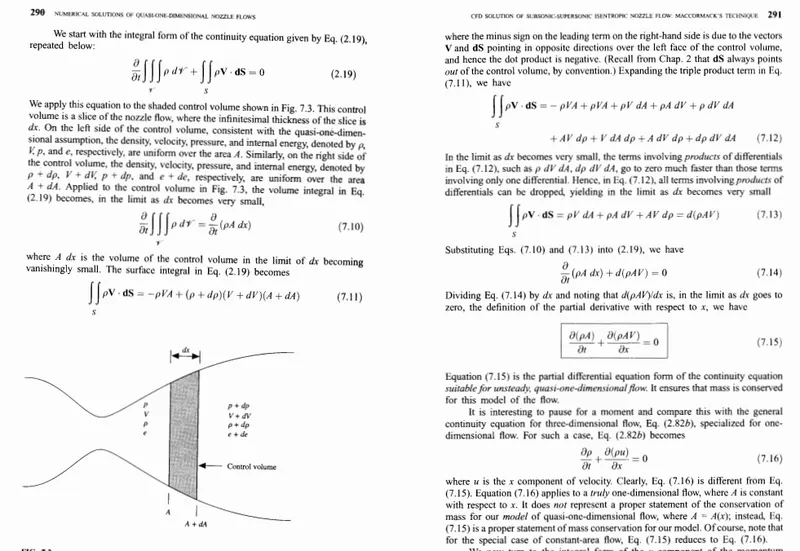
both the x and y directions. This is the real physics of the flow. On the other hand, the assumption of quasi-one-dimensional flow dictates that the flow properties are functions of x only. Since this assumption twists the real physics of the flow, then Eqs. (2.82) to (2.86) are not necessarily appropriate for quasi-one-dimensional flow. On the other hand, for the equations that are appropriate for quasi-one-dimensional flow, we would at least like for the overall physical principles of (I) mass conservation, (2) Newton's second law, and (3) energy conservation to hold exactly, in spite of our twisted physics due to the quasi-one-dimensional assumption. To ensure that these physical principles are satisfied, we must return to the integral forms of the governing equations derived in Chap. 2 and apply these integral forms to a control volume consistent with the quasi-one-dimensional assumption. Let us proceed.
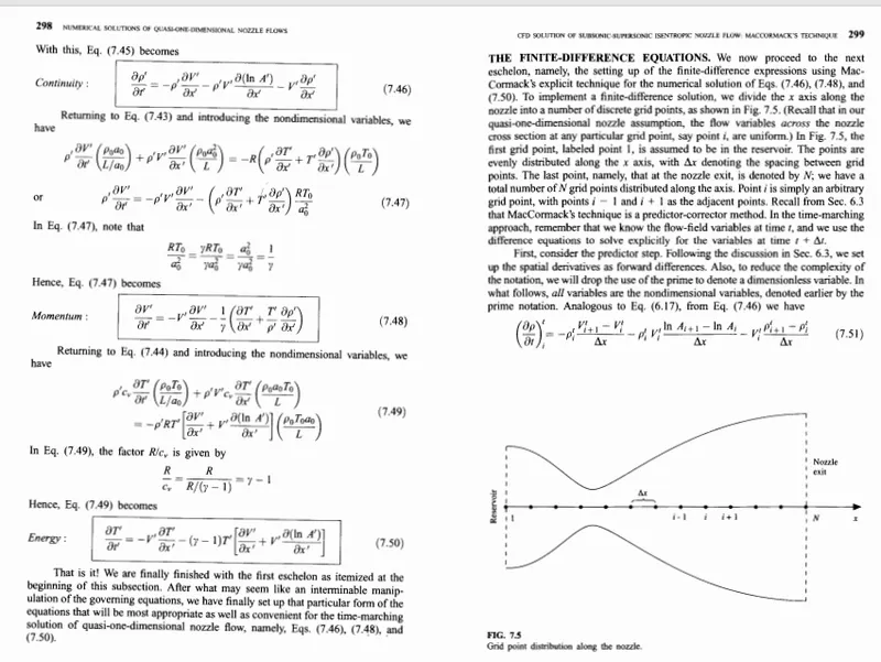
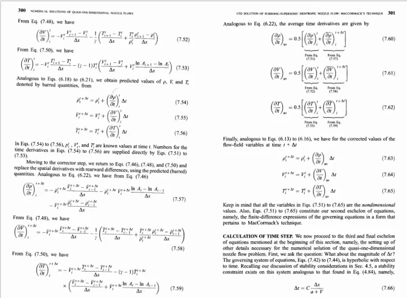
THIS CAN BE SOLVED VIA 2 DISTINCT PROCESS. ONE IS CONSERVATIVE PROCESS AND OTHER IS NON CONSERVATIVE PROCESS
FIRST WE ARE GOING TO SHOW AND CODE FOR NON-CONSERVATIVE PROCESS.
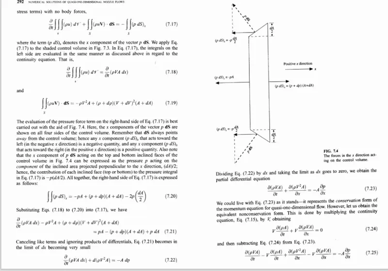
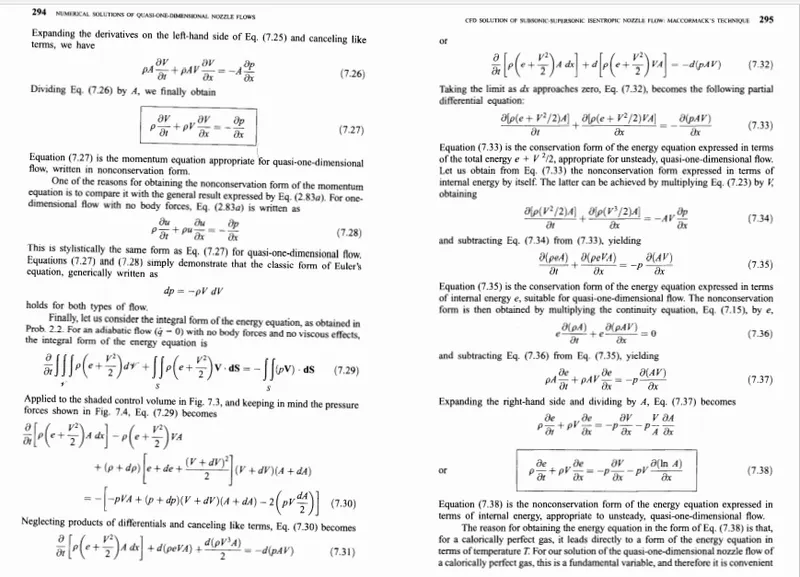
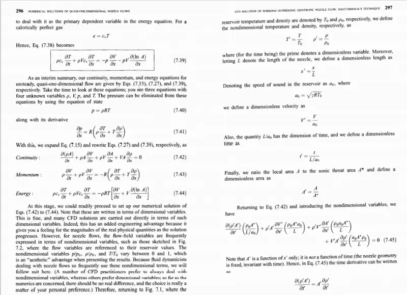
THE EQUATIONS ARE ATTACHED IN THE IMAGE BELOW.
PLEASE FOLLOW THE PAGE NUMBER OF THE FOLLOWING IMAGES TO UNDERSTAND THE EQUATIONS.
NOW WE ARE GOING TO CODE THIS ABOVE NON-CONSERVATIVE PROCESS
clear all
close all
clc
SPECIFYING THE GRID SPACING
n=31;
%SPECIFYING THE LENGTH OF THE NOZZLE i.e x
x=linspace(0,3,n);
%finding the difference of length between two gridpoints
dx=x(2)-x(1);
gamma=1.4;
%DEFINING THE VARIABLES IN THE INITIAL STATE
%THESE POINTS ARE OBTAINED BY NON DIMENTIONALIZING THE DIMENTIONALIZED
%TERMS.
%DENSITY
rho=1-0.3146*x;
%TEMPERATURE
t=1-.2314*x;
%VELOCITY
v=(0.1+1.03*x).*t.^0.5;
%AREA
a=1+2.2*(x-1.5).^2;
%timesteps loop
%DEFINING THE NUMBER OF TIMELOOP FOR WHICH THE ITERATIONS WILL GO ON.
nt=1400;
%C IS THE COURANT NUMBER
c=0.5;
%CALCULATING THE DIFFRENCE BETWEEN TWO CONSQUITIVE VALUES.
%THIS IS COMPUTED WITH THE BELOW FORMULAE AND SELECTING THE MINIMUM VALUE.
dt=min(c.*dx./(sqrt(t)+v));
%FOR NON CONSERVATIVE EQUATIONS
%HERE I HAVE CREATED A FUNCTION TO SOLVE THE NON CONSERVATIVE PROCESS.
%THE PROCESS FOLLOWED IS ATTACHED IN THE REPORT FOR FURTHER REFERENCES.
%THE NAME OF THE FUNCTION IS "non_conservative_func"
[rho,v,t,p,machno,mfr]=non_conservative_func(n,x,dx,gamma,rho,t,v,a,nt,c,dt);
%FOR CONSERVATIVE EQUATIONS
%HERE I HAVE CREATED A FUNCTION TO SOLVE THE CONSERVATIVE PROCESS.
%THE PROCESS FOLLOWED IS ATTACHED IN THE REPORT FOR FURTHER REFERENCES.
%THE NAME OF THE FUNCTION IS "conservative_func"
a1=1+2.2*(x-1.5).^2;
mt=1400;
c1=0.5;
[rho1,v1,t1,p1,machno1,mfr1]=conservative_func(n,x,dx,gamma,a1,nt,c1,dt);
%HERE WE ARE PLOTTING THE MASS FLOW RATE OF BOTH THE CONSERVATIVE AND
%NON-CONSERVATIVE PROCESS WITH RESPECT TO THE RELATIVE NOZZLE LENGTH.
figure(29)
plot(x,mfr1)
hold on
plot(x,mfr)
xlabel('x/L')
ylabel('NON DIMENSIONAL MASS FLOW RATE MFR/MFR0')
grid on
THE ABOVE CODE IS ATTACHED BELOW. THIS IS THE MAIN CODE CONTAINING THE FUNCTIONS.
clear all
close all
clc


%SPECIFYING THE GRID SPACING
n=31;
%SPECIFYING THE LENGTH OF THE NOZZLE i.e x
x=linspace(0,3,n);
%finding the difference of length between two gridpoints
dx=x(2)-x(1);
gamma=1.4;

%DEFINING THE VARIABLES IN THE INITIAL STATE
%THESE POINTS  ARE OBTAINED BY NON DIMENTIONALIZING THE DIMENTIONALIZED
%TERMS.
%DENSITY
rho=1-0.3146*x;
%TEMPERATURE
t=1-.2314*x;
%VELOCITY
v=(0.1+1.03*x).*t.^0.5;
%AREA
a=1+2.2*(x-1.5).^2;

%timesteps loop
%DEFINING THE  NUMBER OF TIMELOOP  FOR WHICH THE ITERATIONS WILL GO ON.
nt=1400;
%C IS THE COURANT NUMBER
c=0.5;
%CALCULATING THE DIFFRENCE BETWEEN TWO CONSQUITIVE VALUES.
%THIS IS COMPUTED WITH THE BELOW FORMULAE AND SELECTING THE MINIMUM VALUE.
dt=min(c.*dx./(sqrt(t)+v));

                            %FOR NON CONSERVATIVE EQUATIONS

%HERE I HAVE CREATED A FUNCTION TO SOLVE THE NON CONSERVATIVE PROCESS.
%THE PROCESS FOLLOWED IS ATTACHED IN THE REPORT FOR FURTHER REFERENCES.

%THE NAME OF THE FUNCTION IS "non_conservative_func"


[rho,v,t,p,machno,mfr]=non_conservative_func(n,x,dx,gamma,rho,t,v,a,nt,c,dt);


                         %FOR CONSERVATIVE EQUATIONS

%HERE I HAVE CREATED A FUNCTION TO SOLVE THE CONSERVATIVE PROCESS.
%THE PROCESS FOLLOWED IS ATTACHED IN THE REPORT FOR FURTHER REFERENCES.


%THE NAME OF THE FUNCTION IS "conservative_func"

a1=1+2.2*(x-1.5).^2;
mt=1400;
c1=0.5;


 [rho1,v1,t1,p1,machno1,mfr1]=conservative_func(n,x,dx,gamma,a1,nt,c1,dt);


 %HERE WE ARE PLOTTING THE MASS FLOW RATE OF BOTH THE CONSERVATIVE AND
 %NON-CONSERVATIVE PROCESS WITH RESPECT TO THE RELATIVE NOZZLE LENGTH.
 figure(29)
 plot(x,mfr1)
 hold on
 plot(x,mfr)
 xlabel('x/L')
 ylabel('NON DIMENSIONAL MASS FLOW RATE MFR/MFR0')
 grid on
WE HAVE FORMED FUNCTION FOR BOTH CONSERVATIVE AND NON CONSERVATIVE PROCESS
FIRST GET FAMILIARIZED WITH NON CONSERVATIVE PROCESS.
THE CODE IS ATTACHED WITH COMMENT FOR BETTER UNDERSTANDING.
 function [rho,v,t,p,machno,mfr]=non_conservative_func(n,x,dx,gamma,rho,t,v,a,nt,c,dt)


%outer time loop
%HERE WE ARE STARTING THE TIME MARCHING LOOP SO  THAT WE CAN FIND OUT HOW
%THE FLOW THROUGH THE SUPERSONIC NOZZLE HAPPENS OVER TIMES.

for k=1:nt

    %HERE WE ARE JUST KEEPING THE RECORDS OF rho ,t,v in some variable for
    %cross referencing in latter period of time.
    rho_old=rho;
    v_old=v;
    t_old=t;


    %SINCE WE ARE USING MACCORMAC'S METHOD HENCE WE NEED TO COMPUTE
    %PREDICTOR AND CORRECTOR STEP TO FIND THE DESIRED VALUE OF THE NON
    %DIMENTIONAL QUANTITIES.

    %PREDICTOR TERMS
    for j=2:n-1

        %HERE WE HAVE BROKEN DOWN THE TERMS OF THE continuity
        %equation,momentum equation,energy equation.HERE WE ARE USING
        %FOREWORD DIFFERENCE TO FIND THE DESIRED VALUES OF FIRST
        %DERIVATIVES WRT x
        dvdx=(v(j+1)-v(j))/dx;
        drhodx=(rho(j+1)-rho(j))/dx;
        dtdx=(t(j+1)-t(j))/dx;
        dlogadx=(log(a(j+1))-log(a(j)))/dx;

        %continuity equation
        drhodt_p(j)=  -(rho(j)*dvdx) - (rho(j)*(v(j)*dlogadx))- (v(j)*drhodx);
        %momentum equation
        dvdt_p(j)=    -(v(j)*dvdx) - ((1/gamma)*((dtdx) + ((t(j)/rho(j))*drhodx)));
        %energy equation
        dtdt_p(j)=    -(v(j)*dtdx) -  (gamma-1)*t(j)*((dvdx+ (v(j)*dlogadx)));


        %solution update
        %THE ONLY NEED TO UPDATE THE VALUE IS BECAUSE WE NEED TO FIND OUT VALUES OF PRIMITIVE VARIABLES TO UPDATE CORRECTOR TERMS.
        rho(j)=rho(j)+drhodt_p(j)*dt;
        v(j)=v(j)+dvdt_p(j)*dt;
        t(j)=t(j)+dtdt_p(j)*dt;
    end


    %corrector term
    %HERE WE STAND TO 2ND STEP OF MCCORMAC'S METHOD.
    %WE PROCEED WITH THE  COMPUTATION OF THE CORRECTOR TERMS.

    for j=2:n-1

        %HERE WE HAVE BROKEN DOWN THE TERMS OF THE continuity equation,momentum equation,energy equation.HERE WE ARE USING
        %REARWARD DIFFERENCE TO FIND THE DESIRED VALUES OF FIRST
        dvdx=(v(j)-v(j-1))/dx;
        drhodx=(rho(j)-rho(j-1))/dx;
        dtdx=(t(j)-t(j-1))/dx;
        dlogadx=(log(a(j))-log(a(j-1)))/dx;

        %continuity equation
        drhodt_c(j)=      -(rho(j)*dvdx) - (rho(j)*(v(j)*dlogadx))- (v(j)*drhodx);
        %momentum equation
        dvdt_c(j)=    -(v(j)*dvdx) - ((1/gamma)*((dtdx) + ((t(j)/rho(j))*drhodx)));
        %energy equation
        dtdt_c(j)=        -(v(j)*dtdx) -  (gamma-1)*t(j)*((dvdx+ (v(j)*dlogadx)));


    end

     %The average time derivatives are formed as follows.
    drhodt=0.5*(drhodt_p+drhodt_c);
    dvdt=0.5*(dvdt_p+dvdt_c);
    dtdt=0.5*(dtdt_p+dtdt_c);

%    AFTER FINDING THE AVERAGE TIME DERIVATIVES OF THE PRIMITIVE VARIABLES
%    The final corrected values of rho , t, and v at time step t+dt (here, since t = O
%    to start with, we are calculating the final corrected values at time t=dt) are obtained from
    for i=2:n-1
      rho(i)=rho_old(i)+drhodt(i)*dt;
        v(i)=v_old(i)+dvdt(i)*dt;
        t(i)=t_old(i)+dtdt(i)*dt;

    end


    %specifying boundary condition.

    % rho , t, and v  boundary conditions changes according to the BC given in the textbook.
    %SINCE WE ARE COMPUTING VALUES FROM N=2 TO NTH TERM HENCE WE NEED TO
    %EXTRAPOLATE THE VALUES OF N=1 AND N=N
    %inlet
    v(1)=2*v(2)-v(3);

    %outlet
    rho(n)=2*rho(n-1)-rho(n-2);
    v(n)=2*v(n-1)-v(n-2);
    t(n)=2*t(n-1)-t(n-2);
    p=rho.*t;
    machno=v./t.^2;
    mfr=rho.*a.*v;


            %         plotting  nozzle length graphs
%
        figure(1)
        plot(x,v)
        title(sprintf('NON CONSERVATIVE PROCESS:timestep=%d',k))
        pause(0.00003)
        xlabel('x/L')
        ylabel('NON DIMENSIONAL VELOCITY v/v0')
        legend('RELATIVE VELOCITY VARIATION WITH NOZZLE LENGTH')


        figure(2)
        plot(x,rho)
        title(sprintf('NON CONSERVATIVE PROCESS:timestep=%d',k))
        pause(0.00003)
        xlabel('x/L')
        ylabel('NON DIMENSIONAL DENSITY rho/rho0')
        legend('RELATIVE DENSITY VARIATION WITH NOZZLE LENGTH')


        figure(3)
        plot(x,t)
        title(sprintf('NON CONSERVATIVE PROCESS:timestep=%d',k))
        pause(0.00003)
        xlabel('x/L')
        ylabel('NON DIMENSIONAL TEMPERATURE t/t0')
        legend('RELATIVE TEMPERATURE VARIATION WITH NOZZLE LENGTH')

        figure(4)
        plot(x,machno)
        title(sprintf('NON CONSERVATIVE PROCESS:timestep=%d',k))
        pause(0.00003)
        xlabel('x/L')
        ylabel('NON DIMENSIONAL mach no m/m0')
        legend('RELATIVE MACHNO VARIATION WITH NOZZLE LENGTH')

        figure(5)
        plot(x,p)
        title(sprintf('NON CONSERVATIVE PROCESS:timestep=%d',k))
        pause(0.00003)
        xlabel('x/L')
        ylabel('NON DIMENSIONAL pressure p/p0')
        legend('RELATIVE PRESSURE VARIATION WITH NOZZLE LENGTH')


%     %         time marching graph sectioN


        figure(6)
        plot(k,v(16),'.','color','r','markersize',10)
        hold on
        title(sprintf('NON CONSERVATIVE PROCESS:timestep=%d',k))
        xlabel('t')
        ylabel('NON DIMENSIONAL VELOCITY v/v0')
        axis([0 1500 0.5 1.4])
        pause(0.0003)
        legend('RELATIVE VELOCITY VARIATION WITH TIMESTEP')

        figure(7)
        plot(k,rho(16),'.','color','r','markersize',10)
        hold on
        title(sprintf('NON CONSERVATIVE PROCESS:timestep=%d',k))
        xlabel('t')
        ylabel('NON DIMENSIONAL DENSITY RHO/RHO0')
        axis([0 1500 0.5 1])
        pause(0.0003)
        legend('RELATIVE DENSITY VARIATION WITH TIMESTEP')


        figure(8)
        plot(k,t(16),'.','color','g','markersize',10)
        hold on
        title(sprintf('NON CONSERVATIVE PROCESS:timestep=%d',k))
        xlabel('t')
        ylabel('NON DIMENSIONAL TEMPERATURE temp/temp0')
        axis([0 1500 0.65 .95])
        pause(0.0003)
        legend('RELATIVE TEMPERATURE VARIATION WITH TIMESTEP')


        figure(9)
        plot(k,p(16),'.','color','g','markersize',10)
        hold on
        title(sprintf('NON CONSERVATIVE PROCESS:timestep=%d',k))
        xlabel('t')
        ylabel('NON DIMENSIONAL PRESSURE pressur/pressur0')
        axis([0 1500 0.3 .95])
        pause(0.0003)
        legend('RELATIVE PRESSURE VARIATION WITH TIMESTEP')


        figure(10)
        plot(k,machno(16),'.','color','b','markersize',10)
        hold on
        title(sprintf('NON CONSERVATIVE PROCESS:timestep=%d',k))
        xlabel('t')
        ylabel('NON DIMENSIONAL MACHNO machno/machno0')
        axis([0 1500 0.95 3.4])
        pause(0.0003)
        legend('RELATIVE MACH NO VARIATION WITH TIMESTEP')

    mass flow rate vs relative length
            figure(11)
           plot(x,mfr)
           title(sprintf('NON CONSERVATIVE PROCESS:timestep=%d',k))
           xlabel('x/L')
         ylabel('NON DIMENSIONAL MASS FLOW RATE MFR/MFR0')
         pause(0.0003)

        figure(123)
        plot(k,mfr(16),'.','color','b','markersize',10)
        hold on
        title(sprintf('NON-CONSERVATIVE PROCESStimestep=%d',k))
        xlabel('t')
        ylabel('NON DIMENSIONAL MFR mfr/mfr0')
        axis([0 1500 0 1.3])
        pause(0.0003)


end


end
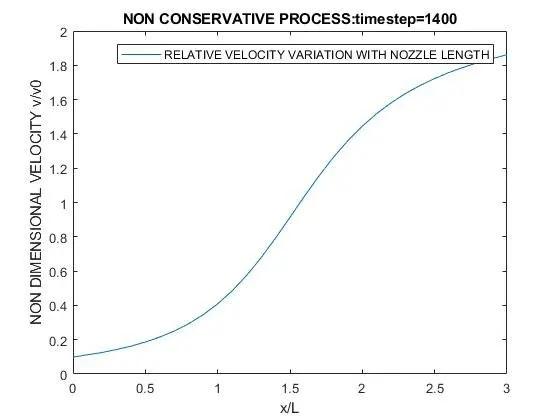
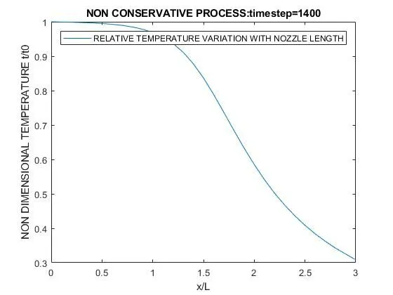
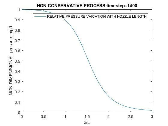
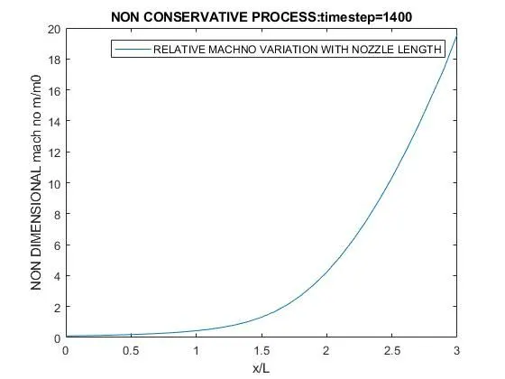
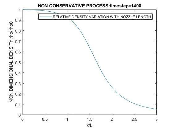
THE GRAPHS FOR Steady-state distribution of primitive variables inside the nozzle are as follows.-FOR NON-CONSERVATIVE PROCESS
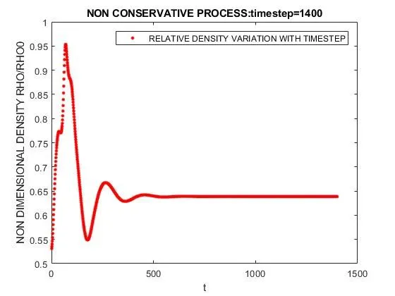
THE GRAPHS FORTime-wise variation of the primitive variables-FOR NON-CONSERVATIVE PROCESS
FIRST GET FAMILIARIZED WITH CONSERVATIVE PROCESS.
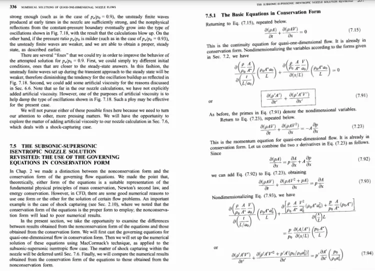
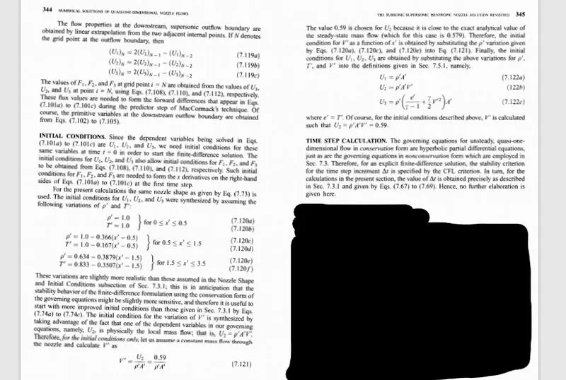
THE SUBSONIC-SUPERSONICISENTROPIC NOZZLE SOLUTION REVISITED: THE USE OF THE GOVERNING EQUATIONS IN CONSERVATION FORM
In Chap. 2 we made a distinction between the nonconservation form and the conservation form of the governing flow equations. We made the point that, theoretically, either form of the equations is a suitable representation of the fundamental physical principles of mass conservation, Newton's second law, and energy conservation. However, in CFD, there are some good numerical reasons to use one form or the other for the solution of certain flow problems. An important example is the case of shock capturing (see Sec. 2.10), where we noted that the
conservation form of the equations is the proper form to employ; the nonconservation form will lead to poor numerical results. In the present section, we take the opportunity to examine the differences between results obtained from the nonconservation form of the equations and those obtained from the conservation form. We will first cast the governing equations for quasi-one-dimensional flow in conservation form. Then we will set up the numerical solution of these equations using MacCormack's technique, as applied to the subsonic-supersonic isentropic flow case. The matter of shock capturing within the nozzle will be deferred until Sec. 7.6. Finally, we will compare the numerical results obtained from the conservation form of the equations to those obtained from the nonconservation form.
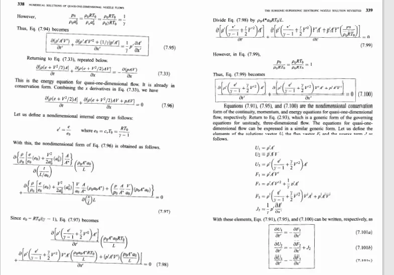
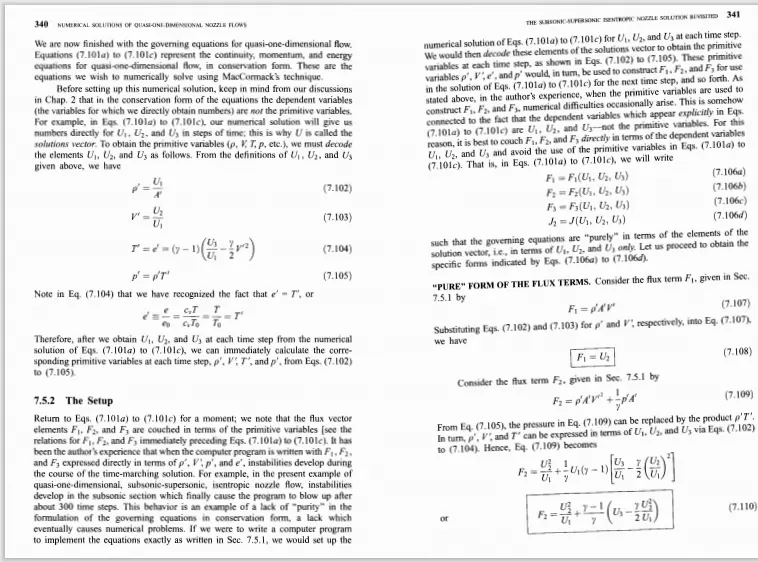
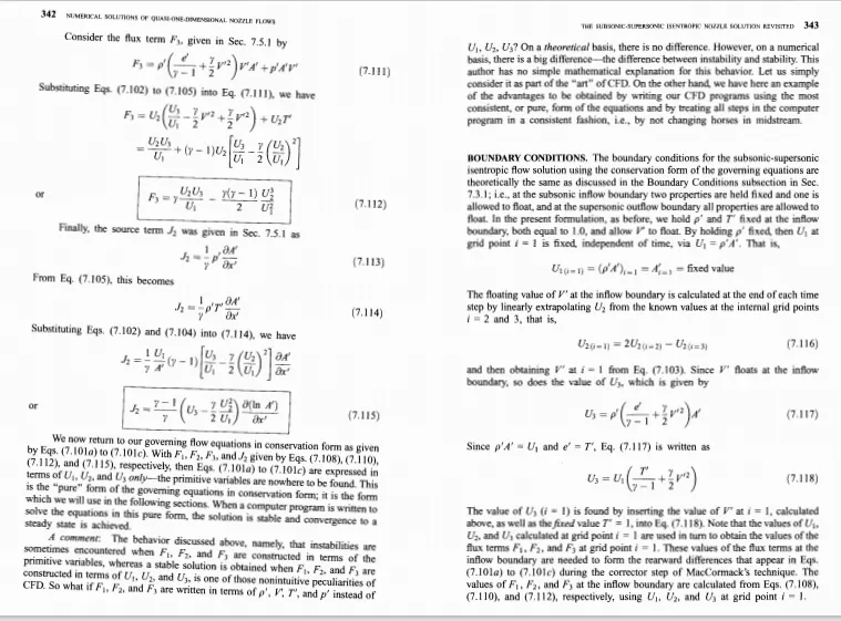
THE DETAILED THEORY IS ATTACHED BELOW FOR BETTER CORELATION.
THE CODE IS ATTACHED WITH COMMENT FOR BETTER UNDERSTANDING.
function [rho1,v1,t1,p1,machno1,mfr1]=conservative_func(n,x,dx,gamma,a1,nt,c1,dt)

for i=1:length(x)

    % This is the syntax for conditional operator.
    %IF THE VALUE OF x IS BETWEEN 0AND 0.5 THEN THE VALUE OF  rho1 and t1 are as follows.
    if x(i)>= 0 && x(i)<= 0.5
        rho1(i)=1;
        t1(i)=1;
     %IF THE VALUE OF x IS BETWEEN 0.5 AND 1.5 THEN THE VALUE OF  rho1 and t1 are as follows.

    elseif x(i)>=0.5 && x(i)<=1.5
        rho1(i)=1-0.366*(x(i)-0.5);
        t1(i)=1-0.167*(x(i)-0.5);

    %IF THE VALUE OF x IS BETWEEN 1.5 AND 3.0  THEN THE VALUE OF  rho1 and t1 are as follows.
    elseif x(i)>=1.5 && x(i)<= 3.0
        rho1(i)=0.634-0.3879*(x(i)-1.5);
        t1(i)=0.833-0.3507*(x(i)-1.5);

    end
    % rho1 should be indexed.
    %since we have found the value of rho1 and t wecan use that value to find velocity v1 using the obtained  data
    v1(i)=0.590./(rho1(i).*a1(i));
end

%Equations  are the nondimensional conservation form of the continuity, momentum, and energy equations for quasi-one-dimensional flow, respectively. Return to Eq. (2.93), which is a generic form of the governing
%equations for unsteady, three-dimensional flow. The equations for quasi-onedimensional flow can be expressed in a similar generic form.
%Let us define the elements of the solutions vector U, the flux vector F, and the source term J as follows

%this defining u1 u2 u3 first.
u1=rho1.*a1;
u2=rho1.*a1.*v1;
u3=rho1.*a1.*((t1/(gamma-1))+0.5*gamma.*v1.^2);

%DEFINING THE  NUMBER OF TIMELOOP  FOR WHICH THE ITERATIONS WILL GO ON.
mt=1400;
%C IS THE COURANT NUMBER
c1=0.5;
%CALCULATING THE DIFFRENCE BETWEEN TWO CONSQUITIVE VALUES.
%THIS IS COMPUTED WITH THE BELOW FORMULAE AND SELECTING THE MINIMUM VALUE.
dt=min(c1.*dx./(sqrt(t1)+v1));


%HERE WE ARE STARTING THE TIME MARCHING LOOP SO  THAT WE CAN FIND OUT HOW
%THE FLOW THROUGH THE SUPERSONIC NOZZLE HAPPENS OVER TIMES.

for g=1:1400;

    % these terms have to be inside the loop so that the they update after
    % each time step
    u1_old=u1;
    u2_old=u2;
    u3_old=u3;

    % Same her as well. If weare caluclating the f1,f2 and f3 from updated u1,u2 and u3 F1 F2 F3 ARE THE FLUX TERMS.
    %THESE VALUES WILL BE UPDATED AFTER EACH TIMELOOP.

    f1=u2;
    f2=(u2.^2./u1)+((gamma-1)/gamma).*(u3-(0.5*gamma).*(u2.^2./u1));
    f3=gamma.*(u2.*u3./u1)-(gamma*(gamma-1)*.5.*(u2.^3./u1.^2));

    %SINCE WE ARE USING MACCORMAC'S METHOD HENCE WE NEED TO COMPUTE
    %PREDICTOR AND CORRECTOR STEP TO FIND THE DESIRED VALUE OF THE NON
    %DIMENTIONAL QUANTITIES.

    %PREDICTOR TERMS


    for z=2:n-1

        %Note that by using THE BELOW EQUATION for J2 rather than the expression given IN TEXT BOOK.
        %we are breaking slightly with the purity. of the governing.The results are not compromise.
        j2(z)=rho1(z).*t1(z).*(a1(z+1)-a1(z))/(gamma*dx);

        % The predicted time derivatives of U1, U2 , and _u3 are obtained respectively, using FOREWARD differences for the x derivatives.

        du1dt_p(z)=-(f1(z+1)-f1(z))/dx;             %  value matched with textbook
        du2dt_p(z)=-((f2(z+1)-f2(z))/dx)+j2(z);    %  value matched with textbook
        du3dt_p(z)=-(f3(z+1)-f3(z))/dx;            %  value matched with textbook

         %solution update
        %THE ONLY NEED TO UPDATE THE VALUE IS BECAUSE WE NEED TO FIND OUT VALUES OF PRIMITIVE VARIABLES TO UPDATE FLEX TERMS.
        u1(z)=u1(z)+du1dt_p(z)*dt;
        u2(z)=u2(z)+du2dt_p(z)*dt;
        u3(z)=u3(z)+du3dt_p(z)*dt;
        %
    end


    %AFTER WE ARE PREDICTOR TERMS WE RE FINDING THE VALUES  OF PRIMITIVE
    %TERMS SO THAT WE CAN UPDATE THE VALUES OF THE FLEX TERMS.
    rho1=u1./a1;
    t1=(gamma-1)*((u3./u1)-(gamma*0.5.*(u2./u1).^2));
    v1=u2./u1;
    p1=rho1.*t1;

    %updating the flex terms.
    %THE UPDATED FLEX TERMS ARE REQUIRED TO  COMPUTE THE CORRECTOR TERMS FOR FURTHER CORRECT DATA.
    f1=u2;
    f2=(u2.^2./u1)+((gamma-1)/gamma)*(u3-(0.5*gamma).*(u2.^2./u1));
    f3=gamma.*(u2.*u3./u1)-(gamma*(gamma-1)*.5.*(u2.^3./u1.^2));


    %CORRECTOR TERMS


    %HERE WE STAND TO 2ND STEP OF MCCORMAC'S METHOD.
    %WE PROCEED WITH THE  COMPUTATION OF THE CORRECTOR TERMS.

    for z=2:n-1

        % The CORRECTED time derivatives of U1, U2 , and _u3 are obtained respectively, using rearward differences for the x derivatives.


        du1dt_c(z)=-(f1(z)-f1(z-1))/dx;                                                   %  value matched with textbook
        du2dt_c(z)=-((f2(z)-f2(z-1))/dx)+ (rho1(z).*t1(z).*(a1(z)-a1(z-1))/(gamma*dx)) ;  %  value matched with textbook
        du3dt_c(z)=-(f3(z)-f3(z-1))/dx;                                                   %  value matched with textbook

    end
    %The average time derivatives are formed as follows.
    du1dt_a=0.5*(du1dt_p+du1dt_c);
    du2dt_a=0.5*(du2dt_p+du2dt_c);
    du3dt_a=0.5*(du3dt_p+du3dt_c);


%AFTER FINDING THE AVERAGE TIME DERIVATIVES OF THE SOLUTION VECTORS WE
%UPDATING THE VALUE SOF U1 U2 AND U3.
%The final corrected values of U1 , U2 , and U3 at time step t+dt (here, since t = O
%to start with, we are calculating the final corrected values at time t=dt) are obtained from
    for l=2:n-1
        u1(l)=u1_old(l)+du1dt_a(l)*dt;
        u2(l)=u2_old(l)+du2dt_a(l)*dt;
        u3(l)=u3_old(l)+du3dt_a(l)*dt;

    end


    %mentionig the boundery conditions
    % u1,u2, u3 boundary conditions changes according to the BC given in the textbook.
    %SINCE WE ARE COMPUTING VALUES FROM N=2 TO NTH TERM HENCE WE NEED TO
    %EXTRAPOLATE THE VALUES OF N=1 AND N=N
    %  u1(1)=2*u1(2)-u1(3);
    u1(1) = rho1(1).*a1(1);
    u2(1)=2*u2(2)-u2(3);
    %  u3(1)=2*u3(2)-u3(3);
    u3(1)=u1(1)*(t1(1)/(gamma-1)+(gamma/2)*v1(1).^2);

    u1(n)=2*u1(n-1)-u1(n-2);
    u2(n)=2*u2(n-1)-u2(n-2);
    u3(n)=2*u3(n-1)-u3(n-2);

    %now debugging the u1 u2 and u3
    %THE  PREMITIVE VARIABLE ARE AS FOLLOWS.


    rho1=u1./a1;
    v1=u2./u1;
    t1=(gamma-1).*((u3./u1)-(gamma*0.5.*(u2./u1).^2));
    p1=rho1.*t1;
    machno1=v1./t1.^2;
    mfr1=rho1.*a1.*v1;

%         plotting  nozzle length graphs

        figure(15)

        plot(x,v1)
        title(sprintf('CONSERVATIVE PROCESS:timestep=%d',g))
        pause(0.00003)
        xlabel('x/L')
        ylabel('NON DIMENSIONAL VELOCITY v/v0')
        legend('RELATIVE VELOCITY VARIATION WITH NOZZLE LENGTH')
        pause(0.000003)
        grid on

        figure(16)

        plot(x,rho1)
        title(sprintf('CONSERVATIVE PROCESS:timestep=%d',g))
        pause(0.00003)
        xlabel('x/L')
        ylabel('NON DIMENSIONAL DENSITY rho/rho0')
        legend('RELATIVE DENSITY VARIATION WITH NOZZLE LENGTH')
        pause(0.000003)


        figure(17)

        plot(x,t1)
        title(sprintf('CONSERVATIVE PROCESS:timestep=%d',g))
        pause(0.00003)
        xlabel('x/L')
        ylabel('NON DIMENSIONAL TEMPERATURE t/t0')
        legend('RELATIVE TEMPERATURE VARIATION WITH NOZZLE LENGTH')
        pause(0.000003)

        figure(18)

        plot(x,machno1)
        title(sprintf('CONSERVATIVE PROCESS:timestep=%d',g))
        pause(0.00003)
        xlabel('x/L')
        ylabel('NON DIMENSIONAL mach no m/m0')
        legend('RELATIVE MACH NO VARIATION WITH NOZZLE LENGTH')
        pause(0.000003)

        figure(19)

        plot(x,p1)
        title(sprintf('CONSERVATIVE PROCESS:timestep=%d',g))
        pause(0.00003)
        xlabel('x/L')
        ylabel('NON DIMENSIONAL pressure p/p0')
        legend('RELATIVE PRESSURE VARIATION WITH NOZZLE LENGTH')
        pause(0.000003)


% %         time marching graph sectioN
%

        figure(20)
        plot(g,v1(16),'.','color','r','markersize',10)
        hold on
        title(sprintf('CONSERVATIVE PREOCESS: timestep=%d',g))
        xlabel('t')
        ylabel('NON DIMENSIONAL VELOCITY v/v0')
        axis([0 1500 0.8 1])
        legend('RELATIVE VELOCITY VARIATION WITH TIMESTEP')
        pause(0.0003)

        figure(21)
        plot(g,rho1(16),'.','color','r','markersize',10)
        hold on
        title(sprintf('CONSERVATIVE PREOCESS:timestep=%d',g))
        xlabel('t')
        ylabel('NON DIMENSIONAL DENSITY RHO/RHO0')
        axis([0 1500 0.6 .7])
        legend('RELATIVE DENSITY VARIATION WITH TIMESTEP')
        pause(0.0003)

        figure(22)
        plot(g,t1(16),'.','color','g','markersize',10)
        hold on
        title(sprintf('CONSERVATIVE PREOCESS:timestep=%d',g))
        xlabel('t')
        ylabel('NON DIMENSIONAL TEMPERATURE temp/temp0')
        axis([0 1500 0.8 0.9])
        legend('RELATIVE TEMPERATURE VARIATION WITH TIMESTEP')
        pause(0.0003)

        figure(23)
        plot(g,p1(16),'.','color','g','markersize',10)
        hold on
        title(sprintf('CONSERVATIVE PREOCESS:timestep=%d',g))
        xlabel('t')
        ylabel('NON DIMENSIONAL PRESSURE pressur/pressur0')
        axis([0 1500 0.45 .62])
        legend('RELATIVE PRESSURE VARIATION WITH TIMESTEP')
        pause(0.0003)

        figure(24)
        plot(g,machno1(16),'.','color','b','markersize',10)
        hold on
        title(sprintf('CONSERVATIVE PREOCESS:timestep=%d',g))
        xlabel('t')
        ylabel('NON DIMENSIONAL MACHNO machno/machno0')
        axis([0 1500 .2 .4])
        legend('RELATIVE MACH NO VARIATION WITH TIMESTEP')
        pause(0.0003)


        figure(124)
        plot(g,mfr1(16),'.','color','b','markersize',10)
        hold on
        title(sprintf('CONSERVATIVE PROCESS-timestep=%d',g))
        xlabel('t')
        ylabel('NON DIMENSIONAL MFR mfr/mfr0')
        axis([0 1500 0 1.3])
        pause(0.0003)

end


end
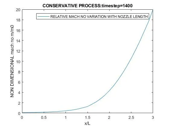
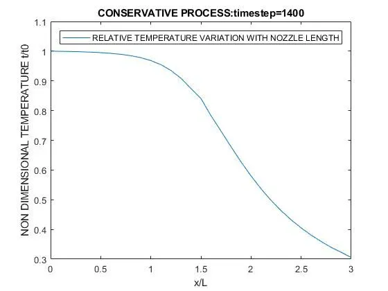
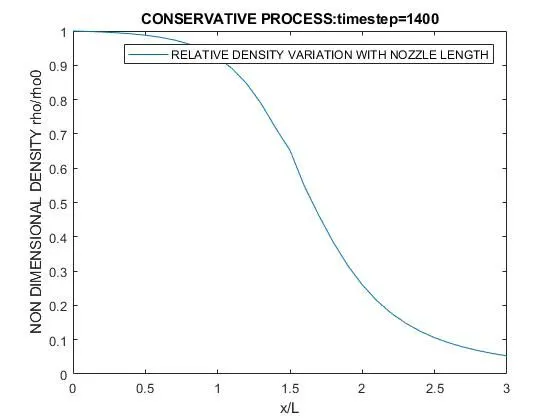
THE GRAPHS FOR Steady-state distribution of primitive variables inside the nozzle are as follows.
FOR CONSERVATIVE PROCESS
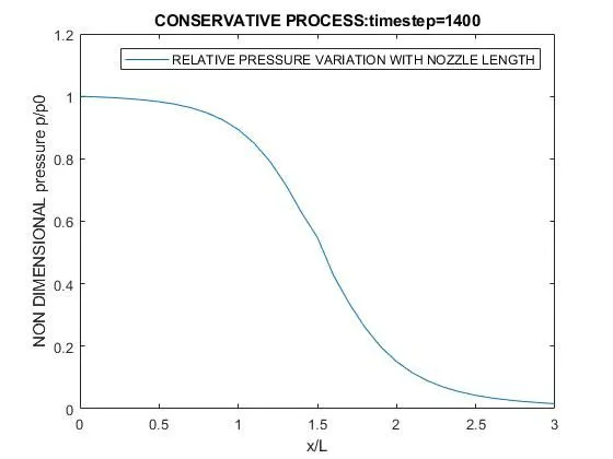
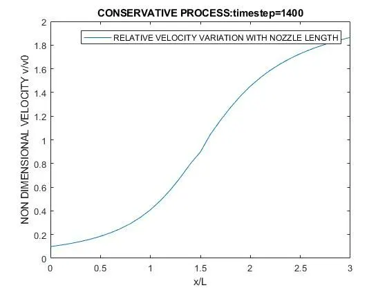
THE GRAPHS FOR Time-wise variation of the primitive variables-FOR CONSERVATIVE PROCESS
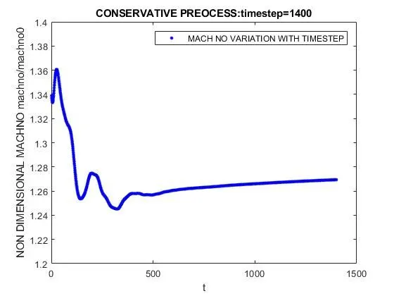
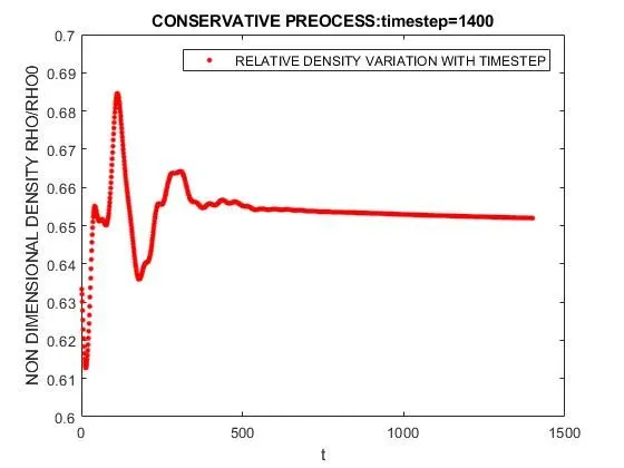
THE ABOVE PROGRAM IS GRID INDEPENDENT.SO WHATEVER BE THE NUMBER OF GRID THE SOLUTION WILL ALWAYS BE THE SAME.
Variation of Mass flow rate distribution inside the nozzle at different time steps during the time-marching process
1.NON-CONSERVATIVE PROCESS.
2.CONSERVATIVE PROCESS.
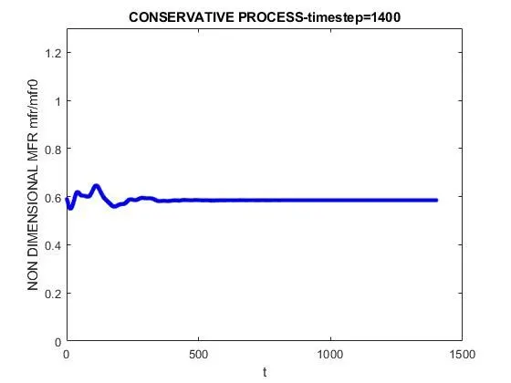
Comparison of Normalized mass flow rate distributions of both forms
CONCLUSION
FROM THIS PROJECT WE HAVE CONCLUDED THAT WHATEVER BE THE GRIDSPACING THE RESULTS ARE INDIPENDENT OF THE GRIDSIZE.ALSO FOR CONSERVATIBE AND NON CONSERVATIVE THE RELATIVE VELOCITY,TEMPERATURE,DENSITY,MACHNO,PRESSURE AND MASS FLOW RATE REMAINS MORE OR LESS SAME .