Week 9 - FVM Literature Review
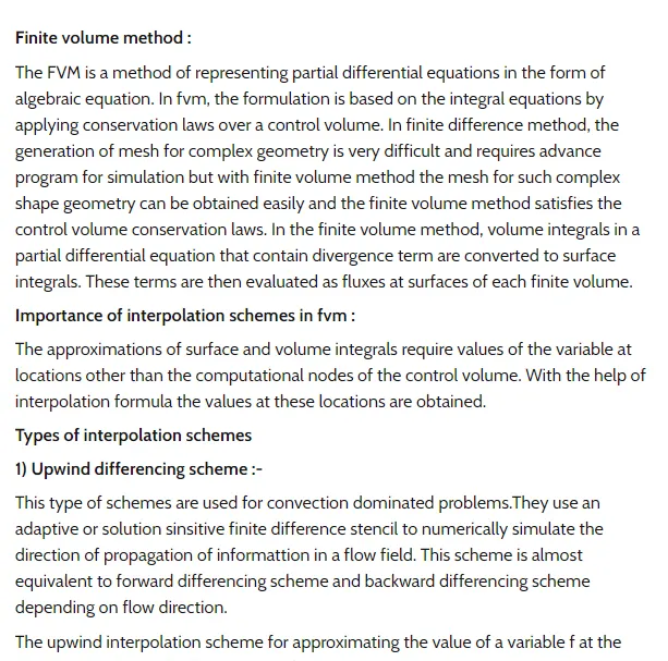
The finite volume method (FVM) is a method for representing and evaluating partial differential equations in the form of algebraic equations. In the finite volume method, volume integrals in a partial differential equation that contain a divergence term are converted to surface integrals, using the divergence theorem. These terms are then evaluated as fluxes at the surfaces of each finite volume. Because the flux entering a given volume is identical to that leaving the adjacent volume, these methods are conservative. Another advantage of the finite volume method is that it is easily formulated to allow for unstructured meshes. The method is used in many computational fluid dynamics packages. "Finite volume" refers to the small volume surrounding each node point on a mesh.
Finite volume methods can be compared and contrasted with the finite difference methods, which approximate derivatives using nodal values, or finite element methods, which create local approximations of a solution using local data, and construct a global approximation by stitching them together. In contrast a finite volume method evaluates exact expressions for the average value of the solution over some volume, and uses this data to construct approximations of the solution within cells.
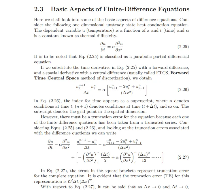
Finite Differences
Finite Differences
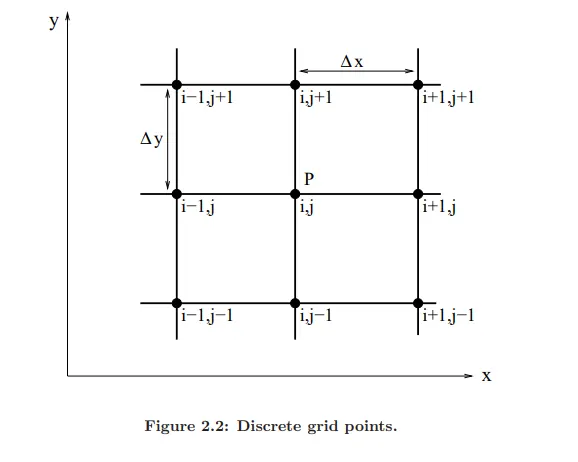
Analytical solutions of partial differential equations provide us with closed-form expressions which depict the variation of the dependant variables in the domain. The numerical solutions, based on finite differences, provide us with the values at discrete points in the domain which are known as grid points. Consider Fig. 2.2, which shows a domain of calculation in the x − y plane. Let us assume that the spacing of the grid points in the x−direction is uniform, and given by ∆x. Likewise, the spacing of the points in the y−direction is also uniform, and given by ∆y. It is not necessary that ∆x or ∆y be uniform. We could imagine unequal spacing in both directions, where different values of ∆x between each successive pairs of grid points are used. The same could be presumed for ∆y as well. However, often, problems are solved on a grid which involves uniform spacing in each direction, because this simplifies the programming, and often results in higher accuracy. In some class of problems, the numerical calculations are performed on a transformed computational plane which has uniform spacing in the transformed-independent-variables, but non-uniform spacing in the physical plane. These typical aspects will be discussed later in the Chapter on grid generation. In the present chapter we shall consider uniform spacing in each coordinate direction. According to our consideration, ∆x and ∆y are constants, but it is not mandatory that ∆x be equal to ∆y. Let us once again refer to Fig. 2.2. The grid points are identified by an index i which increases in the positive x-direction, and an index j, which increases in the positive y-direction. If (i, j) is the index of point P in Fig. 2.2, then the point immediately to the right is designated as (i+ 1, j) and the point immediately to the left is (i−1, j). Similarly the point directly above is (i, j + 1), and the point directly below is (i, j − 1). The basic philosophy of finite difference methods is to replace the derivatives of the governing equations with algebraic difference quotients. This will result in a system of algebraic equations which can be solved for the dependant variables at the discrete grid points in the flow field. Let us now look at some of the common algebraic difference quotients in order to be acquainted with the methods related to discretization of the partial differential equations.
Finite Volume Method
The Finite Difference Method for solving differential equations is simple to understand and implement. However, it has one significant drawback: it can only be applied to meshes in which the cell faces are lined up with the coordinate axes. As such, it becomes difficult, if not out outright impossible, to resolve curved boundaries – like those encountered when dealing with any realistic geometry.
The Finite Volume Method (FVM) offers an alternative approach for deriving the discretized equations. This method is based on the principle that the divergence term, that frequently occurs in differential equations governing various interesting scientific phenomena, can be rewritten as a surface integral using the divergence theorem. The problem then simplifies to evaluating fluxes normal to the cell walls. Since this becomes a vector problem, the cell walls can take any shape and can be arbitrarily oriented. All that is required is that the they enclose a closed volume. And since the method is based on evaluating fluxes, the Finite Volume Method is conservative. Outflow from one cell becomes inflow into another. This makes the FVM stable and flexible, and yet relatively easy to implement. This is why the Finite Volume Method is commonly implemented in commercial computational fluid dynamics (CFD) solvers.
The Finite Volume Method
Consider the general Poisson equation, the governing equation in electrostatics, but also in other areas such as gas diffusion: ∇2ϕ=b∇2ϕ=b
In electrostatics, the right hand side is the negative charge density divided by the electrical permitivity. In diffusion, it becomes the species production rate. We can write this equation in the integral form by integrating both sides over some control volume. We then get
∫V∇⋅∇ϕdV=∫VbdV∫V∇⋅∇ϕdV=∫VbdV
r by employing the Divergence Theorem and assuming the value of the right hand side is constant over the control volume
∮S∇ϕ⋅^ndA=~bΔV∮S∇ϕ⋅n^dA=b~ΔV
where ΔVΔV is the volume of the control volume. Finally, we can approximate the integral on the left hand side by summing over the faces of our control volume. Assuming our control volume is a three dimensional Cartesian brick, we obtain (Eq. 1)
6∑i=1(∇ϕ)i⋅(^ndA)i=~bΔxΔyΔz(1)
Example
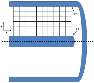
As an example, let’s consider the potential between two conducting cylinders shown in Figure 1. The domain of interest is the empty space with an annular geometry. This problem is both simpler and more complicated than the case presented in Eq. 1. It is simpler because if we assume the problem is axi-symmetric (quite a valid assumption), the problem becomes two dimensional. But it is more complex however since we are now dealing with the cylindrical coordinate system. But this coordinate system will allow us to better illustrate some of the details of FVM. For now, for simplicity, we will keep the computational mesh rectilinear. We will consider a more general case with arbitrarily shaped cells in a future article.
Potential is governed by the Poisson equation, ∇2ϕ=−ρ/ϵ0∇2ϕ=−ρ/ϵ0 which in cylindrical coordinates is (Eq. 2)
∂2ϕ∂r2+1r∂ϕ∂r+1r2∂2ϕ∂θ2+∂2ϕ∂z2=−ρϵ0(2)
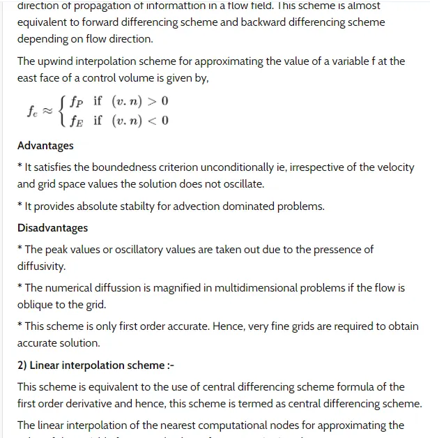
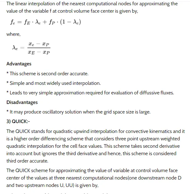
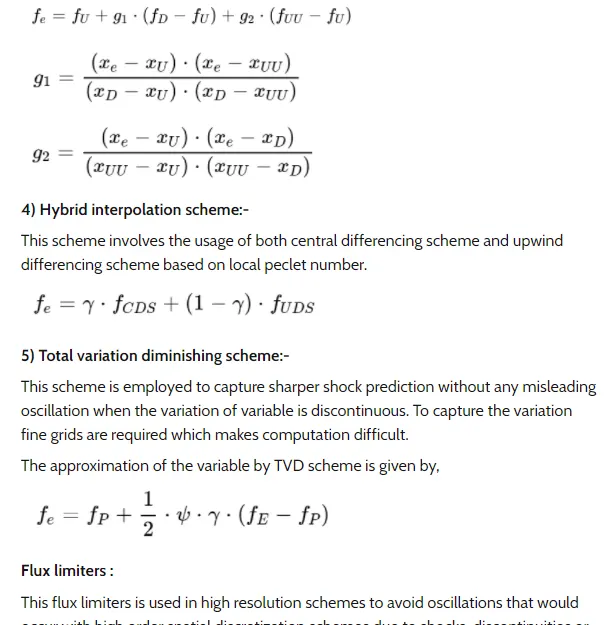
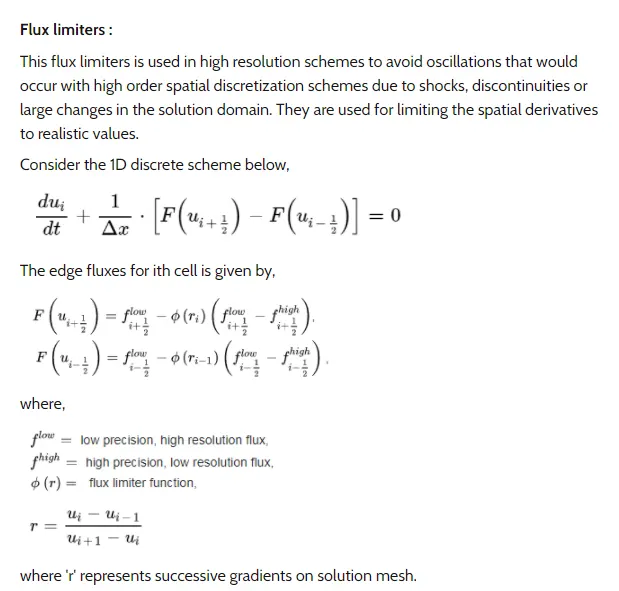
The need for interpolation schemes and flux limiters in FVM