Week 3 - Solving second order ODEs

Aim :

To

1. Write a program in Matlab\Octave that will simulate the pendulum motion, using the following

L=1 metre,

m=1 kg,

b=0.05.

g=9.81 m/s^2.

2. Simulate the motion between 0-20 sec, for angular displacement=0,angular velocity=3 rad/sec at time t=0.

3. Use the information and data obtained to create an animation of the pendulum and upload it to YouTube.

Theory :

In Engineering, ODEs are used to describe the transient behavior of a system. A simple example is a pendulum.

A pendulum is a body suspended from a fixed support such that it swings freely back and forth under the influence of gravity. When a pendulum is displaced sideways from its resting, equilibrium position, it is subject to a restoring force due to gravity that will accelerate it back toward the equilibrium position. When released, the restoring force acting on the pendulum's mass causes it to oscillate about the equilibrium position, swinging it back and forth.

The motion of the pendulum depends on the Newton's second law of motion. When this law is written down, we get a second order Ordinary Differential Equation which describes the position of the "ball" of the pendulum w.r.t time.

The second order ODE used the describe the motion of the pendulum with respect to time is

In the above equation,

g = gravity in m/s2,

L = length of the pendulum in m,

m = mass of the ball in kg,

b=damping coefficient.

Code :

The fixed parameters of the code are as follows

L=1 metre,

m=1 kg,

b=0.05.

g=9.81 m/s2.

Time span = 0-20 sec

Angular displacement=0

Angular velocity=3 rad/sec at time t=0.

The Code for the function ode_solver is given below

function [dtheta_dt] = ode_solver(theta,b,m,g,l)

theta1 = theta(1);
theta2 = theta(2);

dtheta1_dt = theta2; 
dtheta2_dt = -(b/m)*theta2 -(g/l)*sind(theta1);

dtheta_dt = [dtheta1_dt;dtheta2_dt];


end

The above function is used to alot the values of displacement and angular velocity to variables theta1 and theta2 respectively and solve the equations following which they are stored in dtheta_dt as a column matrix.

Code to Solve, Plot and Animate the final results

%Program to solve a second order ODE
clear 
close all
clc

%Defining Constants
b = 0.05;                         %Damping Coefficient
m = 1;                           %Mass of the object (pendulum) - kg
g = 9.81;                        %Acceleration due to gravity - m/s^2
l = 1;                           %Length of pendulum - m

%Defining intial conditions for theta1(displacement) and theta2 (angular velocity)
theta_initial = [0;3];         

%Defining the time interval
t_span = linspace(0,20,200);

%solving the ODE
[t,results] = ode45(@(t,theta) ode_solver(theta,b,m,g,l),t_span,theta_initial);

%Plotting the results
hold on
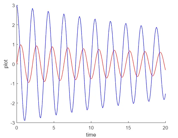
plot(t,results(:,1),'Color','r')
plot(t,results(:,2),'Color','b')
xlabel('time')
ylabel('plot')

%Creating the Animation
ctr = 1
for i = 1:length(results(:,1))
    x0 = 0;
    y0 = 0; 
    x1 = l*sind((results(i,1)*180)/pi)
    y1 = -l*cosd((results(i,1)*180)/pi)
    
    figure(2)
    plot([x0 x1],[y0 y1],'LineWidth',1,'Color','r')
    hold on
    plot(x1,y1,'.','MarkerSize',50,'MarkerFaceColor','auto')
    plot([-1 1],[0 0],"LineWidth",5,'Color',[0 0.4 0])
    axis([-2 2 -2 2]);
    
    M(ctr) = getframe(gcf)
    ctr = ctr+1
    hold off
end

movie(M)
Mov = VideoWriter('Pendulum_motion.avi','Uncompressed AVI')
open(Mov)
writeVideo(Mov,M)
close(Mov)

Results :

The resultant plot between time and Displacement(red) and Angular velocity(blue) is as follows

The YouTube link to the video is given below