Week 4.1 - Genetic Algorithm
Aim :
To
- Write a code in MATLAB to optimise the stalagmite function and find the global maxima of the function.
- Clearly expalin the concept of genetic algorithm in your own words and also explain the syntax for ga in MATLAB.
- Make sure that the code gives the same output, even if it is made to run several times.
- Plot graphs for all 3 studies and for F maximum vs no. of iterations along with the necessary Title and axes labels.
Theory :
Genetic Algorithm (GA) is a search-based optimization technique based on the principles of Genetics and Natural Selection. It is frequently used to find optimal or near-optimal solutions to difficult problems which otherwise would take a lifetime to solve. It is frequently used to solve optimization problems, in research, and in machine learning.
Optimisation is the process of making something better or arriving at a better overall solution to a given problem. Optimization refers to finding the values of inputs in such a way that we get the “best” output values. The definition of “best” varies from problem to problem, but in mathematical terms, it refers to maximizing or minimizing one or more objective functions, by varying the input parameters.
The set of all possible solutions or values which the inputs can take make up the search space. In this search space, lies a point or a set of points which gives the optimal solution. The aim of optimization is to find that point or set of points in the search space.
In Matlab, Genetic Algorithm is an optimisation function, called as ga(), which uses the above mentioned principles of Genetics and Natural selection to find the global minima of a given function.
A Genetic Algorithm goes through 5 phases whilst trying to find the optimum solution for a given function, namely
- Initial population
- Fitness function
- Selection
- Crossover
- Mutation
1. Initial population -
The process begins with a set of individuals which is called a Population. Each individual is a solution to the problem you want to solve.An individual is characterized by a set of parameters (variables) known as Genes. Genes are joined into a string to form a Chromosome (solution).
2. Fitness Function -
The fitness function determines how fit an individual is (the ability of an individual to compete with other individuals). It gives a fitness score to each individual. The probability that an individual will be selected for reproduction is based on its fitness score.
3. Selection -
The idea of selection phase is to select the fittest individuals and let them pass their genes to the next generation. Two pairs of individuals (parents) are selected based on their fitness scores. Individuals with high fitness have more chance to be selected for reproduction.
4. Crossover -
Crossover is the most significant phase in a genetic algorithm. For each pair of parents to be mated, a crossover point is chosen at random from within the genes. Offspring are created by exchanging the genes of parents among themselves until the crossover point is reached. The new offspring are added to the population.
5. Mutation -
In certain new offspring formed, some of their genes can be subjected to a mutation with a low random probability. This implies that some of the bits in the bit string can be flipped. Mutation occurs to maintain diversity within the population and prevent premature convergence.
6. Termination -
The algorithm terminates if the population has converged (does not produce offspring which are significantly different from the previous generation). Then it is said that the genetic algorithm has provided a set of solutions to our problem.
The Syntax of the Genetic algorithm function in Matlab is explained below:

x represents the point of local minima
fun represents the function that is to be optimised, which in our case is the Stalagmite function
nvars represents the number variables used in the function
A and b are used to represent any linear inequalities of the form A*x ≤ b. ga evaluates the matrix product A*x as if x is transposed (A*x').
Aeq and beq are used to represent any linear equalities of the form Aeq*x = beq and A*x ≤ b. ga evaluates the matrix product Aeq*x as if x is transposed (Aeq*x').
lb and ub are used to set the lower and upper bounds for the GA to work within
The function nonlcon accepts x and returns vectors C and Ceq, representing the nonlinear inequalities and equalities respectively. ga minimizes the fun such that C(x) ≤ 0 and Ceq(x) = 0.
options is used to perform additional operations like increasing population size, which is done by using 'optimoptions'
Code :
The code for the stalagmite function is as follows
function [f] = stalagmite(inputs) %inputs is a matrix which
                                  %contains the x and y values

x = inputs(1);
y = inputs(2);

f1x = (sin(5.1*pi*x + 0.5))^6;
f1y = (sin(5.1*pi*y + 0.5))^6;
f2x = exp(-4*(log(2))*(x-0.667)^2/0.64);
f2y = exp(-4*(log(2))*(y-0.667)^2/0.64);

f = -(f1x*f1y*f2x*f2y); %adding a negative sign helps inverse the stalagmite
                      %function so that the GA function can give us the
                      %maximum value for the function
                      %By default GA is a minimisation function.
end
Main Program Code
1. Code to find the optimum function i.e maximum value of Stalagmite function without defining a clear workspace for ga Function.
clear all
close all
clc

%Input Variables
x = linspace(0,0.6,100);
y = linspace(0,0.6,100);

%Creating the workspace
[xx,yy] = meshgrid(x,y);

for i = 1:length(xx(:,1))
    for j = 1:length(yy(:,1))
        input_vector(1) = xx(i,j);
        input_vector(2) = yy(i,j);
        f(i,j) = stalagmite(input_vector);
        freal(i,j) = -f(i,j); % To make the minimum value maximum and vice versa
    end
end

iterations = 50; %Denotes the number of times the genetic algorithm needs to be run
tic %start timer
for i = 1:iterations
    [results,fval(i)] = ga(@stalagmite,2); %here we do not define a workspace for the GA to work within
    x_opt(i) = results(1);
    y_opt(i) = results(2);
    fopt(i) = -fval(i);
end
studytime1 = toc     %End of timer


subplot(2,1,1)
hold on
surfc(xx,yy,freal);        %to Produce a contour plot of the stalagmite function
shading interp;        %To produce a smooth contour without gridlines

plot3(x_opt,y_opt,fopt,'marker','.','MarkerSize',4,'MarkerFaceColor','b') %To plot values of x and y obtained from the ga
                                                                    %function with a blue marker at each point

subplot(2,1,2)
hold on
plot(fopt);              %plotting the optimum value of the stalagmite function after every iteration.
title('Unbounded Workspace');
xlabel('Max F value');
ylabel('Iterations');
Result of the above code
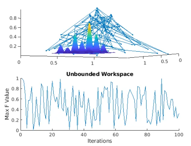
Time taken = 2.7450 secs
As can be seen from the above plots, due to the lack of a particular workspace for the GA to work within, the GA gives very varied results that are scattered all over and very erratic in nature. The above results make it difficult to pinpoint a particular optimal value for the function and is hence not a very useful proposition. The time taken for the study is also less because the number of iterations were limited to just 50.
2. Code to find the optimum function i.e maximum value of Stalagmite function after defining a clear workspace for ga Function. No of iterations has also been increases to 100.
clear all
close all
clc

%Input Variables
x = linspace(0,0.6,100);
y = linspace(0,0.6,100);

%Creating the workspace
[xx,yy] = meshgrid(x,y);

for i = 1:length(xx(:,1))
    for j = 1:length(yy(:,1))
        input_vector(1) = xx(i,j);
        input_vector(2) = yy(i,j);
        f(i,j) = stalagmite(input_vector);
        freal(i,j) = -f(i,j); % To make the minimum value maximum and vice versa
    end
end

iterations = 100; %Denotes the number of times the genetic algorithm needs to be run
tic %start timer
for i = 1:iterations
    [results,fval(i)] = ga(@stalagmite,2,[],[],[],[],[0,0],[0.6,0.6]); %here we do define a lower(0,0) and upper(0.6,0.6)
                                                                       %boundary for the GA to work within
                                                                       % A,b,Aeq,beq have no values and are hence represented by'[]'
    x_opt(i) = results(1);
    y_opt(i) = results(2);
    fopt(i) = -fval(i);
end
studytime1 = toc     %End of timer


subplot(2,1,1)
hold on
surfc(xx,yy,freal);        %to Produce a contour plot of the stalagmite function
shading interp;        %To produce a smooth contour without gridlines

plot3(x_opt,y_opt,fopt,'marker','.','MarkerSize',4,'MarkerFaceColor','b') %To plot values of x and y obtained from the ga
                                                                    %function with a blue marker at each point

subplot(2,1,2)
hold on
plot(fopt);              %plotting the optimum value of the stalagmite function after every iteration.
title('Bounded Workspace');
xlabel('Iterations');
ylabel('Max F Value');
Result of the above code
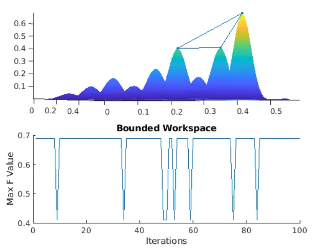
Time taken = 7.0290 secs
The above plots and results show that defining a lower and upperbound i.e, a workspace, for the GA to work within improves the accuracy of the GA and shows us a much narrower range of results. The time taken for the study was a little longer as the number of iterations were increased to 100.
3. Code to find the optimum function i.e maximum value of Stalagmite function, after defining a clear workspace for ga Function and setting a population of 500 for the GA.
clear
close all
clc

%Input Variables
x = linspace(0,0.6,100);
y = linspace(0,0.6,100);

%Creating the workspace
[xx,yy] = meshgrid(x,y);

for i = 1:length(xx(:,1))
    for j = 1:length(yy(:,1))
        input_vector(1) = xx(i,j);
        input_vector(2) = yy(i,j);
        f(i,j) = stalagmite(input_vector);
        freal(i,j) = -f(i,j); % To make the minimum value maximum and vice versa
    end
end

iterations = 100; %Denotes the number of times the genetic algorithm needs to be run
options = optimoptions('ga');
options = optimoptions(options,"PopulationSize",450);

tic %start timer
for i = 1:iterations
    [results,fval(i)] = ga(@stalagmite,2,[],[],[],[],[0,0],[0.6,0.6],[],options);
    %here we do define a lower(0,0) and upper(0.6,0.6)boundary for the GA to work within.
    % A,b,Aeq,beq have no values and are hence represented by'[]'.
    % Options is used to specify or increase the population size of th GA.

    x_opt(i) = results(1);
    y_opt(i) = results(2);
    fopt(i) = -fval(i);
end
studytime1 = toc     %End of timer


subplot(2,1,1)
hold on
surfc(xx,yy,freal);        %to Produce a contour plot of the stalagmite function
shading interp;        %To produce a smooth contour without gridlines

plot3(x_opt,y_opt,fopt,'marker','.','MarkerSize',4,'MarkerFaceColor','b') %To plot values of x and y obtained from the ga
                                                                    %function with a blue marker at each point

subplot(2,1,2)
hold on
plot(fopt);              %plotting the optimum value of the stalagmite function after every iteration.
title('Bounded Workspace with increased population size');
xlabel('Iterations');
ylabel('Max F Value');
Result of the above code
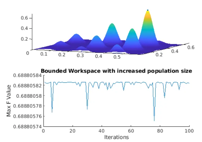
Time taken = 41.4635 secs
From the above results we can see that the GA has reached a solution and given us a pin-pointed accurate optimum solution for the stalagmite function, hence proving that the accuracy of the GA can be much improved by specifying a lower and upper bound as well as by increasing the population size that the GA has to work with. The study time was much longer than the previous iterations because of the increased number of iterations and population size.
Errors :
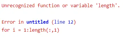
The above error was produced because the object whose length was to be taken into account was not specified.
References :