Centrifugal pump design and analysis

Aim :

To design a centrifugal pump and run an analysis on it to obtain a Performance diagram - the relationship between Pressure ratio and mass flow rate and explain your results.

(Pressure ratio = Outlet total pressure/ Inlet total pressure)

Theory :

A centrifugal pump is a mechanical device designed to move a fluid by means of the transfer of rotational energy from one or more driven rotors, called impellers. Fluid enters the rapidly rotating impeller along its axis and is cast out by centrifugal force along its circumference through the impeller’s vane tips. The action of the impeller increases the fluid’s velocity and pressure and also directs it towards the pump outlet. The pump casing is specially designed to constrict the fluid from the pump inlet, direct it into the impeller and then slow and control the fluid before discharge.

Modelling :

The centrifugal pump designed and modelled using the solidworks software is shown below,

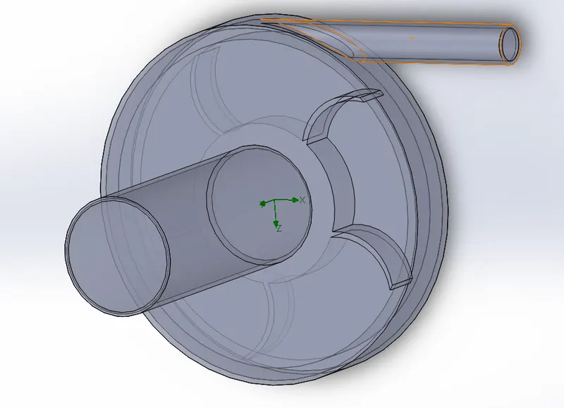
Diameter of Impeller = 40mm

Thickness of Impeller = 10mm

Diameter of Casing = 45mm

Thickness of Casing = 15mm

Inlet diameter = 30mm

Outlet Diameter = 10mm

Simulation and Results :

The Simulation properties and settings were established using the flow simulation wizard.

The fluid used for the simulation was water.

The boundary conditions were given as

Inlet pressure = Environmental Pressure

Outlet Velocity = 10m/s (initial)

Since Solidworks' mesh creation algorithm cannot efficiiently create a moving mesh to simulate the rotation of the impeller, a rotational domain was created encasing the impeller for the sake of conducting the simulation. The velocity assigned to this rotational domain was 1000 rad/s.

A parametric study was conducted to find the change in pressure ratio with change in outlet velocity.

The parametric study was carried out by varying the outlet velocity from a value of 10m/s to 30m/s in incremental steps of 5m/s.

The study was iteration driven i.e. the study ended after the simulator had run 200 iterations.

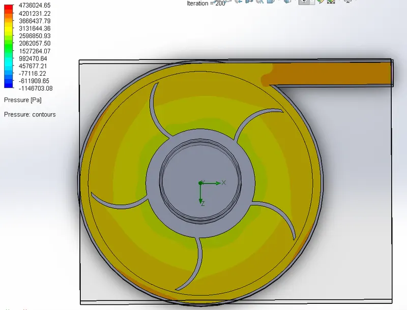
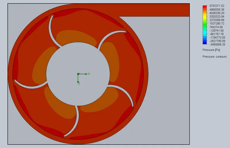
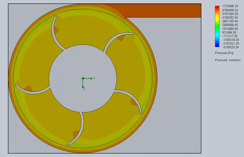
The results of the simulation are given below,

Pressure Plot at 10m/s

Pressure Plot at 15m/s

Pressure Plot at 20m/s

Pressure Plot at 25m/s

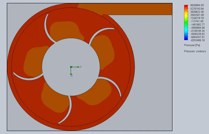
Pressure Plot at 30m/s

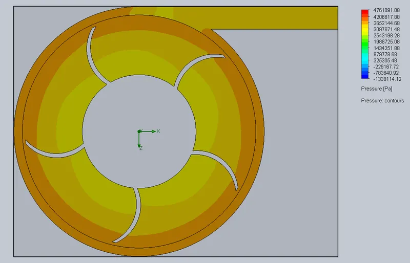
Velocity Plot at 10m/s

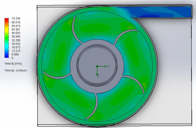
Velocity Plot at 15m/s

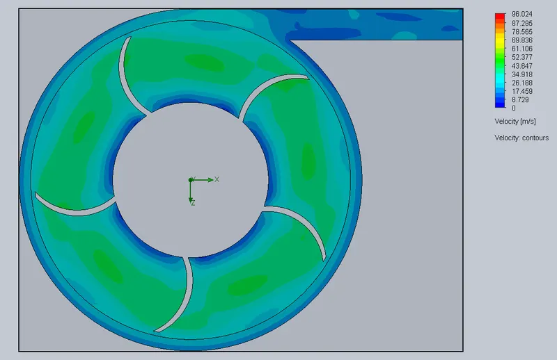
Velocity Plot at 20m/s

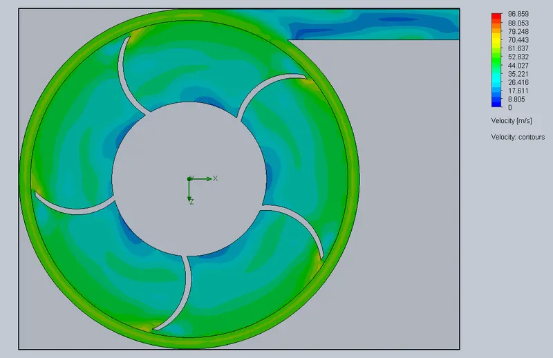
Velocity Plot at 25m/s

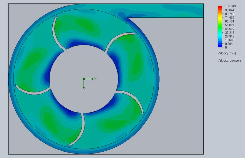
Velocity Plot at 30m/s

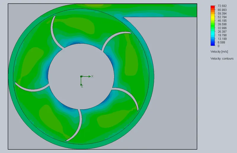
Results of the Simulation :

	10m/s	15m/s	20m/s	25m/s	30m/s
Inlet Pressure (Pa)	246735.80	5191032.44	6525574.39	5301447.31	3726914.34
Outlet Pressure (Pa)	3615176.15	435431.77	435257.76	354791.49	449484.37
Mass Flow rate (Kg/s)	0.4985	0.7472	0.9967	1.2434	1.4955
Pressure Ratio	14.6	11.92	14.99	14.94	8.29

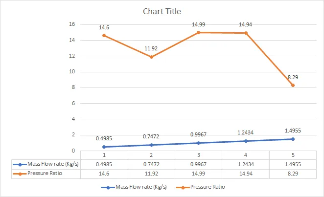
Pressure Ratio Vs Mass Flow Rate Plot

Conclusions :

1. As can be seen from the Cut plots and Graph, as the velocity at the outlet increases, the Mass flow rate at the outlet also increases accordingly.

2. We know that Pressure and velocity are inversely proportional. But the plots do not show much of a reduction in pressure with increase in velocity. This could be due to improper meshing or low computational power to achieve accurate results.

3. So realistically, what we should expect to see from the graphs and plots is a decrease in pressure ratio with an increase in outlet velocity, while the Mass flow rate at the outlet increases with increase in outlet velocity.