Flow over a cylinder

Aim :

To simulate the flow over a cylinder for the conditions shown in the video.

• Calculate the baseline case Reynolds number.
  • Re = rho*U_inlet*D/mu
  • D = cylinder diameter
  • mu = dynamic viscosity
  • rho = density
• Run a baseline simulation and then calculate the Reynolds number. Then increase the Reynolds number by a factor of 20%, 40%, and 100% then run the transient flow simulation.
• Create animations for pressure-velocity for all the three Reynolds number.
• Explain your observations.

Modelling :

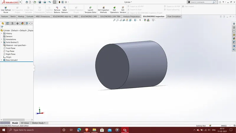
A cylinder of radius 20mm and length 50mm is used for the simulation.

The cylinder is as shown below

The fluid assumed for the external flow simulation was air, the properties of which are given below,

at 15 degrees C

Density of Air = 1.225 kg/m^3

Dynamic Viscosity = 1.8 * 10^-5 kg/ms

We use the above data to calculate the baseline Reynolds Number for the flow simulation.

Assuming a flow Velocity of 10m/s and diameter 0.02m

Baseline Re = 13611

Computational Domain dimensions

+ve X = 0.22m

- ve X = -0.14m

+ve Y = 0.14m

-ve Y = -0.14m

+ve Z = 0.17m

-ve Z = -0.12m

Results and Simulation :

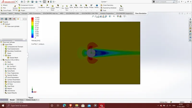
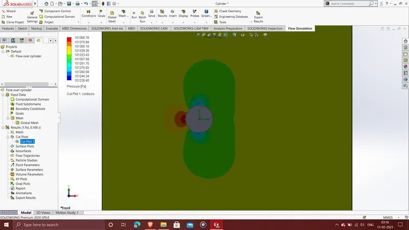
Baseline Simulation :

Length of Domain = 0.36m

Velocity = 10m/s

Flow through time = 0.036 s

End time = 0.072 s

Velocity Cut Plot

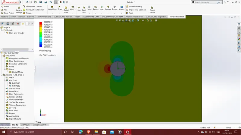
Pressure Cut Plot

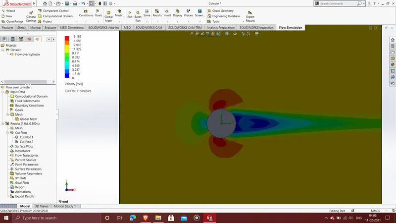
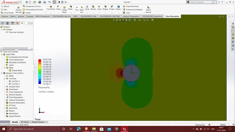
Simulation with 20% increase in Reynold's Number

Re = 16333

Corresponding Flow Velocity = 12m/s

Flow through Time = 0.03s

End time = 0.6s

Velocity Cut Plot

Pressure Cut plot

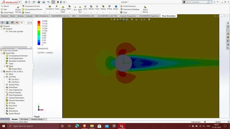
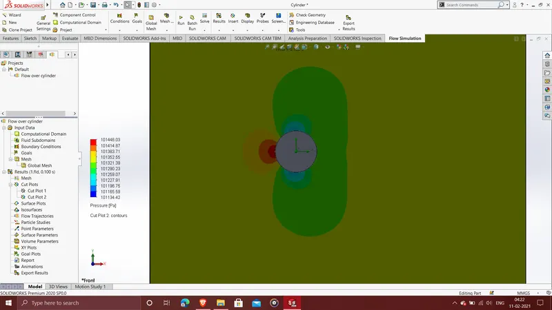
Simulation with 40% increase in Reynold's Number

Re = 19055

Corresponding Flow Velocity = 14m/s

Flow Through Time = 0.026s

End time = 0.052s

Velocity Cut Plot

Pressure Cut Plot

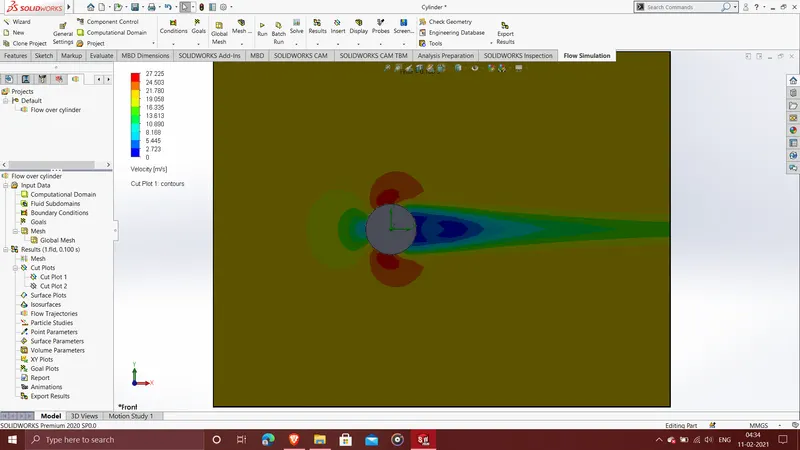
Simulation with 100% increase in Reynold's Number

Re = 27222

Corresponding Flow Velocity = 20m/s

Flow Through Time = 0.018s

End time = 0.036s

Velocity Cut Plot

Pressure Cut plot

Conclusions :

1. The velocity and pressure cut plots look visually similar in all cases.

2. As the Reynolds Number was increased, the velocity and pressure also increases correspondingly, while the flow through time decreases.

3. From the plots its fairly clear that high pressure pockets are formed at regions of low velocity and low pressure pockets are formed at regions of high velocity, thereby showing that velocity and pressure are inversely proportional.