Simulation of pendulum by solving second order ODE using MATLAB

Objective

> A Matlab program to simulate the pendulum motion between 0-20 sec, for angular displacement=0, angular velocity=3 rad/sec at time t=0 using the below given ODE
`(d^2theta)/(dt^2)+(b/m)((d theta)/(dt))+(g/l)sintheta = 0`

> The ODE represents the equation of motion of a simple pendulum with damping where,

g = gravity in m/s^2

L = length of the pendulum in m

m = mass of the ball in kg

b = damping coefficient

Matlab programs

Function program

function [dtheta_dt] = ode_func(t,theta,b,g,L,m)
    theta1 = theta(1)
    theta2 = theta(2)
    dtheta1_dt = theta2;
    dtheta2_dt = -(b/m)*theta2 - (g/L)*sin(theta1);
    dtheta_dt = [dtheta1_dt; dtheta2_dt];
end

Program to simulate and animate the pendulum

clear all
close all
clc

%Input_variables
b=0.05;
g=9.81;
m=1;
L=1;

%Initial_conditions
theta_0 = [0;3];
t_span = linspace(0,20,500);

%ODE_solver
[t,results] = ode45(@(t,theta) ode_func(t,theta,b,g,L,m),t_span, theta_0);
displacement = results(:,1);
velocity = results(:,2);


%Plot
figure(1)
plot(t,[displacement velocity])
xlabel('Time in sec')
ylabel('Angular displacement & Angular velocity in rad/sec')
legend('Angular displacement','Angular velocity')
axis([0 25 -3 3])
grid on


%Pendulum_coordinates
theta = displacement;
ct=1;
for i = 1:length(theta)
    theta1= theta(i);
    x0 = 0;
    y0 = 0;
    
    x1 = L*sin(theta1);
    y1 = -L*cos(theta1);
    
    figure(2)
    plot([-1 1],[0 0],'linewidth',10,'color','k')
    hold on
    plot([x0 x1],[y0 y1],'color','k')
    plot(x1,y1,'o','Markersize',30,'MarkerEdgeColor','r','markerfacecolor','m');
    hold off
    axis ([-1 1 -1.2 .2])
    grid on
    M(ct) = getframe(gcf);
    ct = ct+1;
end

movie(M);
videofile = VideoWriter('Pendulum_animation.avi','Uncompressed AVI');
open(videofile)
writeVideo(videofile,M)
close(videofile)

Program explanation

Function program

> The second order ODE is simplified into two First order ode's.

Let us consider,

`theta = theta1`

`(d(theta))/dt = (d(theta1))/dt=theta2`

Applying above conditions in the given eq,

`(d^2theta)/dt+(b/m)(d theta)/dt+(g/l)sin theta = 0`

`(d^2theta1)/dt+(b/m)(d theta1)/dt+(g/l)sintheta1 = 0`

`(d/dt)theta2+(b/m)theta2+(g/l)sintheta1 = 0`

By simplification we get,

`(d/dt)theta1 = theta2`

`(d/dt)theta2 = -(b/m)theta2-(g/l)sintheta1`

In matrix form,

`(d/dt) [[theta1],[theta2]] = [[theta2],[-(b/m)theta2-(g/l)sintheta1]]`

> Using the above first order ode's the function is defined by which two results, displacement and velocity of the pendulum is obtained.

Simulation and animation program

> The inputs and initial conditions for the simulation of the pendulum is given as

L = 1, m = 1, g = 9.81, b = 0.5, angular displacement=0, angular velocity=3, t = 20s

> Using linspace command the time value is split into 500 samples.

>Then the ODE solver is used to solve the ode's defined in the function and the results are generated

> The result arrays are assigned to variables, displacement and velocity respectively.

> Using plot command the displacement values and velocity values are plotted against time.

> To creat the animation of the pendulum a counter variable (ct) is included with initial value as 1

> By using the below given equations the coordinates of the pendulum is calculated.

`x = l*sintheta`

`y = -l*costheta`

> The coordinates calculated is used to plot the position of the pendulum.

> The plots are stored in an array M(ct) for every loop, using the getframe command.

> Then the ct value is incresed by 1 till the loop ends

> By using the movie command the plots stored in variable M are stitched together.

> Then a videofile with name and format is created

> The videofile created is opened using open command and the writeVideo command is used to write the animation created by the movie command

> By using the close command the videofile is closed.

> The output animation will be the simulation of the pendulum for 20sec with initial angular velocity = 3 rad/sec.

Ode45 syntax explanation

> A numerical ODE solver is used as the main tool to solve the ODE’s.

> The matlab function ode45 will be used.

> ode45 can only solve a first order ODE. Therefore to solve a higher order ODE, the ODE has to be first converted to a set of first order ODE’s.

> This is possible since an n order ODE can be converted to a set of n first order ODE’s.

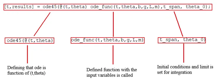
> The above given image shows the syntax of the ODE solver line used in the program

Result of the program

The plot between displacement vs time and velocity vs time is shown below.

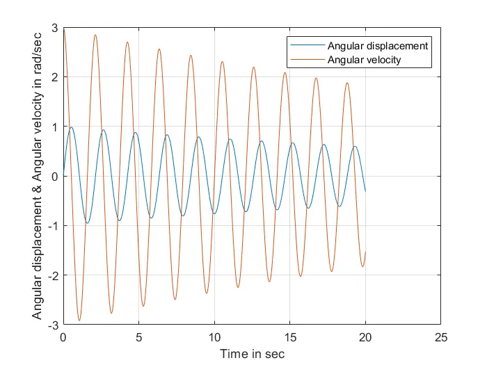
> From the above plot it is seen that the displacement starts from 0 and velocity starts from 3rad/s

> As the time increases the velocity and the displacement decreases due to damping factor.

> The displacement and velocity of the pendulum can be made to 0 within 20secs by increasing the damping coefficient value accordingly.

Pendulum animation link - (https://youtu.be/jgg1OK12O6A)