Optimise Stalagmite function and find global maxima using GA

>x = ga(fun,nvars,A,b) - finds a local minimum x to fun, subject to the linear inequalities A*x ≤ b. ga evaluates the matrix product A*x as if x is transposed (A*x').

>x = ga(fun,nvars,A,b,Aeq,beq) - finds a local minimum x to fun, subject to the linear equalities Aeq*x = beq and A*x ≤ b. (Set A=[] and b=[] if no linear inequalities exist.) ga evaluates the matrix product Aeq*x as if x is transposed (Aeq*x').

>x = ga(fun,nvars,A,b,Aeq,beq,lb,ub) - defines a set of lower and upper bounds on the design variables, x, so that a solution is found in the range lb≤ x ≤ ub. (Set Aeq=[] and beq=[] if no linear equalities exist.)

>x = ga(fun,nvars,A,b,Aeq,beq,lb,ub,nonlcon) - subjects the minimization to the constraints defined in nonlcon. The function nonlcon accepts x and returns vectors C and Ceq, representing the nonlinear inequalities and equalities respectively. ga minimizes the fun such that C(x) ≤ 0 and Ceq(x) = 0. (Set lb=[] and ub=[] if no bounds exist.)

>x = ga(fun,nvars,A,b,Aeq,beq,lb,ub,nonlcon,options) - minimizes with the default optimization parameters replaced by values in options. (Set nonlcon=[] if no nonlinear constraints exist.) Create options using optimoptions.

>x = ga(fun,nvars,A,b,[],[],lb,ub,nonlcon,IntCon,options) - requires that the variables listed in Intcon take integer values.

>x = ga(problem) - finds the minimum for problem, a structure described in problem.

>[x,favl] = ga(___) - for any previous input arguments, also returns fval, the value of the fitness function at x.

function [f] = stalagmite(ip_vector)

x = ip_vector(1);
y = ip_vector(2);

f1 = (sin(5.1*pi*x+0.5)).^6;
f2 = exp(-4*log(2)*((x-0.0667).^2)/0.64);
f3 = (sin(5.1*pi*y+0.5)).^6;
f4 = exp(-4*log(2)*((y-0.0667).^2)/0.64);
f  = -(f1*f2*f3*f4);

% Optimization_using_Genetic_algorithm
close all
clc

% Inputs
x = linspace(0,0.6,150);
y = linspace(0,0.6,150);

% Convertng into 2D array
[xx,yy] = meshgrid(x,y);

% Function call
for i =1:length(xx)
    for j = 1:length(yy)
        ip_vector(1) = xx(i,j);
        ip_vector(2) = yy(i,j);
        f(i,j) = stalagmite(ip_vector);  
    end
end

% Plotting stalagmite func
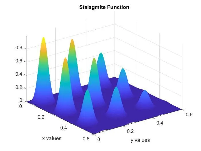
surfc(xx,yy,-f)
shading interp
xlabel('x values')
ylabel('y values')
title('Stalagmite Function')

% ------------------------------------------------------------------------------

% Study 1 - Statistical behaviour
tic
iter = 50;
for i = 1:iter
    [inputs,fopt(i)] = ga(@stalagmite,2);
    xopt(i) = inputs(1);
    yopt(i) = inputs(2);
end
 Studytime1 = toc
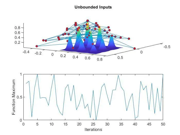
 figure(2)
 subplot(2,1,1)
 hold on
 surfc(x,y,-f)
 shading interp
 title('Unbounded Inputs')
 plot3(xopt,yopt,-fopt,'marker','o','markersize',5,'markerfacecolor','r')
 subplot(2,1,2)
 plot(-fopt)
 xlabel('Iterations')
 ylabel('Function Maximum')
    
% ------------------------------------------------------------------------------

% Study 2 - With upper and lower bounds
tic
for i = 1:iter
    [inputs,fopt(i)] = ga(@stalagmite,2,[],[],[],[],[0;0],[0.8;0.8]);
    xopt(i) = inputs(1);
    yopt(i) = inputs(2);
end
 Studytime2 = toc
 figure(3)
 subplot(2,1,1)
 hold on
 surfc(x,y,-f)
 shading interp
 title('UB & LB Inputs')
 plot3(xopt,yopt,-fopt,'marker','o','markersize',5,'markerfacecolor','r')
 subplot(2,1,2)
 plot(-fopt)
 xlabel('Iterations')
 ylabel('Function Maximum')

 % ------------------------------------------------------------------------------
 
 % Study 3 - Increasing GA Iterations
tic
options = optimoptions('ga');
options = optimoptions(options,'populationsize',250)
for i = 1:iter
    [inputs,fopt(i)] = ga(@stalagmite,2,[],[],[],[],[0;0],[0.8;0.8],[],[],options);
    xopt(i) = inputs(1);
    yopt(i) = inputs(2);
end
 Studytime3 = toc
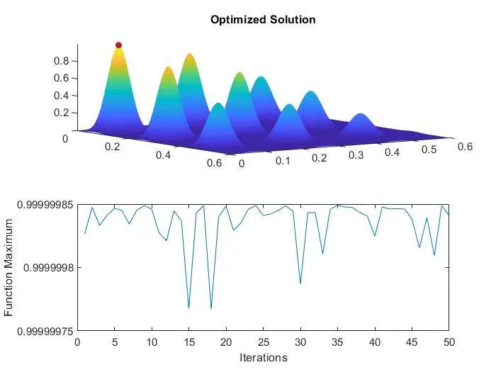
 figure(4)
 subplot(2,1,1)
 hold on
 surfc(x,y,-f)
 shading interp
 title('Optimized Solution')
 plot3(xopt,yopt,-fopt,'marker','o','markersize',5,'markerfacecolor','r')
 subplot(2,1,2)
 plot(-fopt)
 xlabel('Iterations')
 ylabel('Function Maximum')

> The Stalagmite function is written as a seperate code at first

> Since GA calculates the minimum of the a function by default, a minus(-) is multiplied in the stalgamite function to get the maximum value

> Then the x and y ranges are determined in another program which are converted into a 2d array

> The stalagmite function is called and plotted.

> To get the global maxima 3 studies are made

> Unbounded Inputs

> The variable "iter" is included in order to repeat the for loop to get optimal function value (fopt).

> Upper and Lower bounded inputs

> The syntax "x = ga(fun,nvars,A,b,Aeq,beq,lb,ub)" is used inorder to give lower bound(lb) and upper bound(ub) inputs.

> Since there is no linear equalities A, B, Aeq, beq are set to "[]".

> The syntax "x = ga(fun,nvars,A,b,Aeq,beq,lb,ub,nonlcon,options)" is used inorder to increase the initial population size to get the global maxima.

>As there is no linear equalities and nonlinear constraints A, B, Aeq, beq, nonlcon are set to "[]".

> From the three studies it is concluded that with, increased initial population size and input bounds, we can derive optimal solution of the stalagmite function.

> But meanwhile, it will consume more time as it is seen in the workspace image.

> Study3 was 4 times slower than study2.