Parsing NASA thermodynamic data file using MATLAB

Objective

> To write a function that extracts the 14 co-efficients and calculates the enthalpy, entropy and specific heats for all the species in the data file (NASA Thermodynamic data).

> Calculate the molecular weight of each species.

> Plot the Cp, Enthalpy and Entropy for the local temperature range specific for each species.

> Save the plots as images with appropriate names in separate folders for each species automatically.

Program

clear all 
close all 
clc

% Opening the data file
data = fopen('THERMO.dat','r');
H = fgetl(data);

% Converting temperature string to number
temp_data = fgetl(data);
temp_data = strsplit(temp_data,' ');
G_Ltemp = str2num(temp_data{2});
G_Mtemp = str2num(temp_data{3});
G_Htemp = str2num(temp_data{4});

% Excluding comment lines
fgetl(data);
fgetl(data);
fgetl(data);

% To get coefficients and calculate
for i = 1:53
% Species    
    species = fgetl(data);
    x = strsplit(species,' ');
    s_name = x{1};

% Local Temperatures  
    Ltemp = str2double(x{end-3});
    Mtemp = str2double(x{end-2});
    Htemp = str2double(x{end-1});

% Getting the temp coefficients of the species
    L1 = fgetl(data);
    E = strfind(L1,'E');
    L2 = fgetl(data);
    E = strfind(L2,'E');
    L3 = fgetl(data);
    E = strfind(L3,'E');
    
% Higher temperature coefficients    
    ha1 = str2double(L1(1:12+3));
    ha2 = str2double(L1(12+4:27+3));
    ha3 = str2double(L1(27+4:42+3));
    ha4 = str2double(L1(42+4:57+3));
    ha5 = str2double(L1(57+4:72+3));
    ha6 = str2double(L2(1:12+3));
    ha7 = str2double(L2(12+4:27+3));

% Lower temperature coefficients    
    la1 = str2double(L2(27+4:42+3));
    la2 = str2double(L2(42+4:57+3));
    la3 = str2double(L2(57+4:72+3));
    la4 = str2double(L3(1:12+3)); 
    la5 = str2double(L3(12+4:27+3));
    la6 = str2double(L3(27+4:42+3));
    la7 = str2double(L3(42+4:57+3));

% Temperature array for calculation    
    temp = linspace(Ltemp,Htemp,150);
    R = 8.341;
    
% Calculation of Cp,H and S
    for j = 1:length(temp)
        if temp(j)>= Mtemp
            Cp = (ha1+ ha2.*temp+ ha3.*(temp.^2)+ ha4.*(temp.^3)+ ha5.*(temp.^4)).*R;
            H  = (ha1+ (ha2.*temp)./2+ ha3.*(temp.^2)./3+ ha4.*(temp.^3)./4+ ha5.*(temp.^4)./5+ (ha6./temp)).*(R*temp);
            S  = (ha1*log(temp)+ ha2.*temp+ ha3.*(temp.^2/2)+ ha4.*(temp.^3/3)+ ha5.*(temp.^4/4)+ ha7).*R;
        else 
            Cp = (la1+ la2.*temp+ la3.*(temp.^2)+ la4.*(temp.^3)+ la5.*(temp.^4)).*R;
            H  = (la1+ (la2.*temp)./2+ la3.*(temp.^2)./3+ la4.*(temp.^3)./4+ la5.*(temp.^4)./5+ (la6./temp)).*(R*temp);
            S  = (la1*log(temp)+ la2.*temp+ la3.*(temp.^2/2)+ la4.*(temp.^3/3)+ la5.*(temp.^4/4)+ la7).*R;
        end
    end

% Creating directory
    mkdir(s_name)
    cd(s_name)
% Ploting Temp vs Cp     
    figure(1)
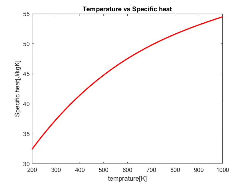
    plot(temp,Cp,'linewidth',2,'color','r');
    xlabel('temprature[K]')
    ylabel('Specific heat[J/kgK]')
    title('Temperature vs Specific heat')
% Ploting Temp vs H
    figure(2)
    plot(temp,H,'linewidth',2,'color','g');
    xlabel('temprature[K]')
    ylabel('Enthalpy[J]')
    title('Temperature vs Specific heat')
% Ploting Temp vs S
    figure(3)
    plot(temp,S,'linewidth',2,'color','b');
    xlabel('temprature[K]')
    ylabel('Entropy[J/K]')
    title('Temperature vs Specific heat')
% Saving the images in the directory
    saveas(figure(1),'Temp vs Specific heat','png');
    saveas(figure(2),'Temp vs Enthalpy','jpeg');
    saveas(figure(3),'Temp vs Entropy','jpeg');
    cd ..
    
% Molecular weight calc
    elements  = ['H','C','N','O','A'];
    at_wt = [1.00784 12.0107 14.0067 15.999 39.948];
    M_Wt = 0;
    
    for i = 1:length(s_name)
        for j = 1:length(elements)
            if strcmp(s_name(i),elements(j))
                M_Wt = M_Wt + at_wt(j);
                x = j;
            end
        end
        n = str2double(s_name(i));
        if n>1
            M_Wt = M_Wt + at_wt(x)*(n-1);
        end
    end
    fprintf('Molecular weight of %s is %f',s_name,M_Wt);
    fprintf('n')
end

Program Logic

Note:

fopen - Used to open the data file

fgetl - Used to get the next line in a data file

strsplit - Used to split a string into cells

strcmp - Used to compare variables

str2num - Used to convert string to number

str2double - Used to convert dtring to double precision values

strfind - Used to get the position of particular element in a string

> fopen command is used to open the data file.

> The second line of the data contains the global temperatures which is assigned to "temp_data" variable using "fgetl".

> The Low,Mid and High temperature values are splitted using "strsplit" and assigned to respective variables.

> The next three lines of the data file are excluded.

> Since there are 53 species a loop for 1:53 is created

> fgetl and strsplit is used to get the name of the species

> The local temperatures of that particular species are assigned respectively

> The next three lines consist the temperature coefficients which are assigned to the respective variable using str2double

> A temperature array is created using linspace command and the gas constant value is assigned to the variable "R"

> A for loop inside a the loop is created to calculate the Cp, H and S values of the species for the temperature array created.

> The temperature array is split into with the medium temperature value using ifelse because, the first seven coefficients are of higher temperature and the next seven are of lower temperature coefficients.

> A directory is is created using mkdir command to save the plots

> Then the plots are generated and saved in the created directory using the saveas command.

> The molecular weight calculation is done using the common species ['H','C','N','O','A'] with their atomic weights [1.00784 12.0107 14.0067 15.999 39.948] respectively

> A for loop is made in which an if statement with strcmp is used to compare the species name and element array.

> If the comparison is true the atomic weight of the corresponding species will be added to the the "M_Wt" varible and the position of the species in the array is stored in variable "x".

> To find species with two or more same elements the species name is assigned to variable "n" using str2double

> Then an if statement is included with condition when n>1, M_Wt = M_Wt + at_wt(x)*(n-1)

> The (n-1) is multiplied because, the atomic weight of the respective element will be added to the molecular weight variable once in the previous loop.

>By using the fprintf command the molecular weight is printed in the command window.

Results

> Plots of O2

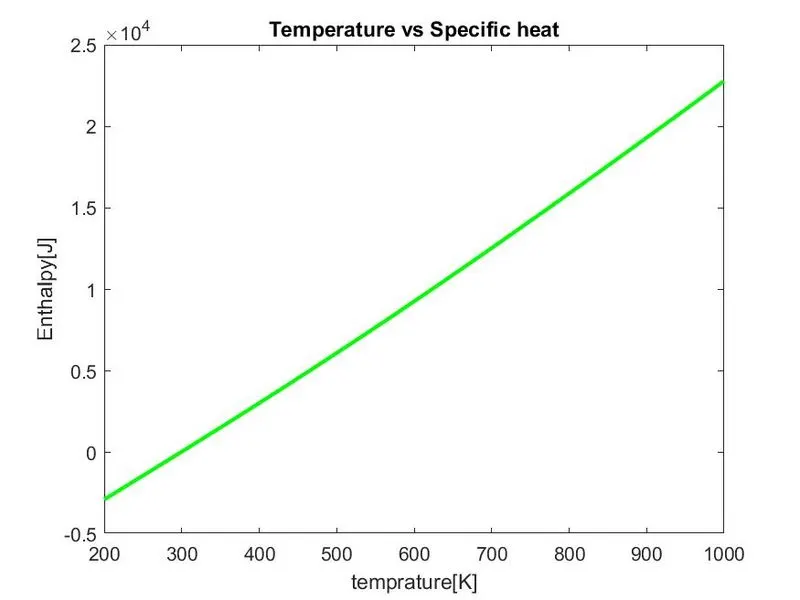
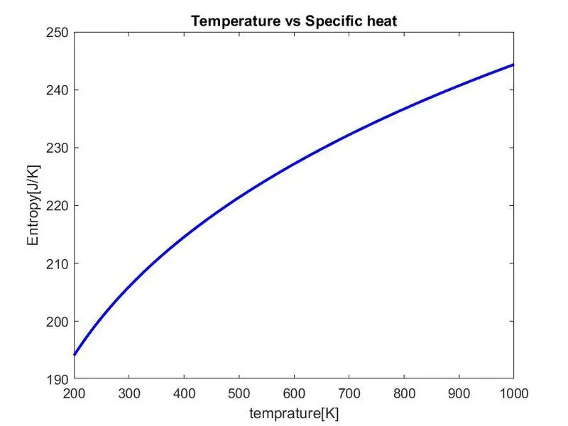
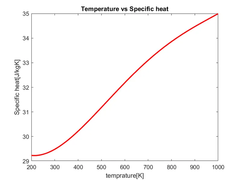
> Plots of N2

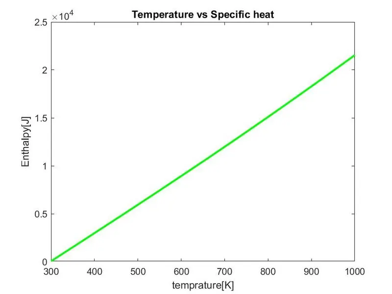
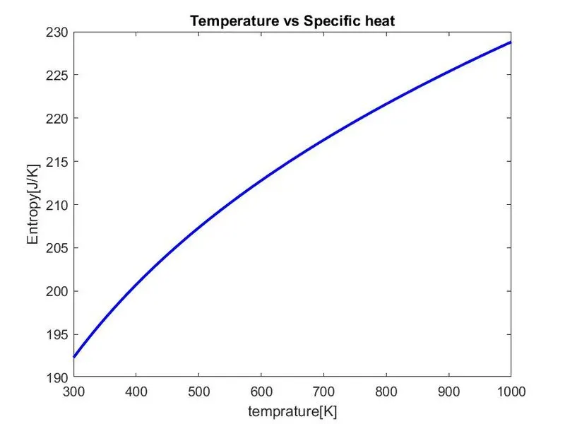
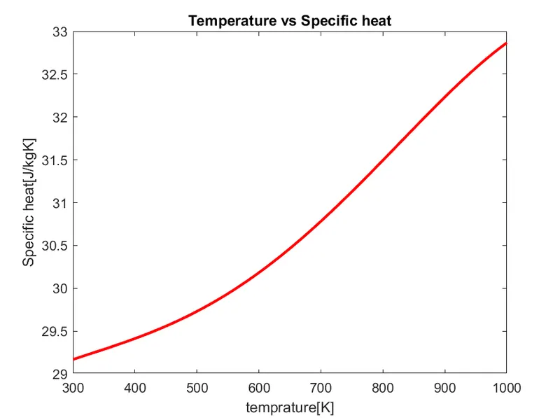
> Plots of CO2

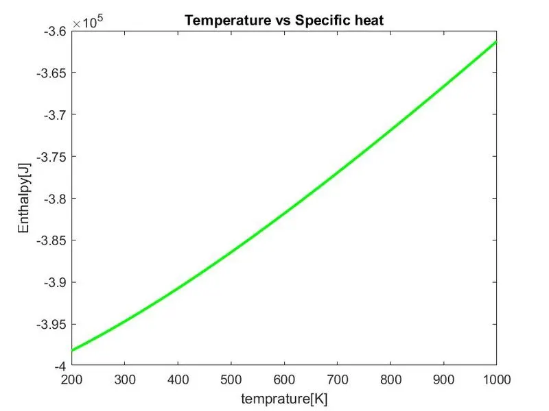
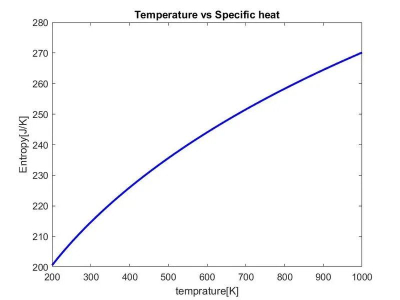
> Screenshot of the window where all the plots are saved