Simulation of air standard cycle using MATLAB

Objective

> To wite a python program to plot the PV diagram and to get the thermal efficiency value of an otto cycle.

Solution procedure

> To plot the PV diagram of the otto cycle it is required to assume the values of some parameters at the state points and engine dimensions to find the values of pressure, temprature and volume at all the state points.

> The assumed parameters are

Bore - 0.1 m P1 - 101325

Storke - 0.1 m T1 - 500 K

Connecting rod - 0.15 m T3 - 2300 K

Compression ratio - 12

> Using the above values the pressure, temprature and volume at all the state points are to be found using formulae.

> Then to calculate the volume points during compression and expanssion process a function is defined in which the volume at diffrent angles of the given range of theta can be calculated.

> To get the pressure points during compression and expanssion the below given formula is used

PV^gamma = constant

> Then all the acquired points can be used to plot the PV diagram of the otto cycle.

> The thermal efficiency of the cycle is calculated using the efficiency formula and then print command is used to print the output to the output window.

Program

#Otto cycle PV plot

#Import req modules
import math
import matplotlib.pyplot as plt


def engine_kinematics(bore,stroke,con_rod,cr,theta_s,theta_e):
	a = stroke/2
	R = con_rod/a

	V_s = (1/4)*math.pi*pow(bore,2)*stroke
	V_c = V_s/(cr-1)

	ts = math.radians(theta_s)
	te = math.radians(theta_e)

	N = 100
	V = []
	for i in range(0,N):
		theta = ts + i*((te-ts)/(N-1))
		term1 = 0.5*(cr-1)
		term2 = R + 1-math.cos(theta)
		term3 = pow((pow(R,2) - pow(math.sin(theta),2)),0.5)

		V.append((1+term1*(term2-term3))*V_c)
	return V

#Inputs
bore    = 0.1
stroke  = 0.1
cr      = 12
con_rod = 0.15
gamma   = 1.4

#Volume parameters
v_s = (1/4)*math.pi*pow(bore,2)*stroke
v_c = v_s/(cr-1)

#State point 1
p1 = 101325
t1 = 500
v1 = v_s+v_c

#State point 2
v2 = v_c
p2 = p1*pow(v1,gamma)/pow(v2,gamma)
t2 = (p2*v2)/((p1*v1)/t1)

#State point 3
t3 = 2300
v3 = v2
p3 = (t3)*(p2/t2)

#State point 4
v4 = v1
p4 = p3*pow(v3,gamma)/pow(v4,gamma) 
t4 = (p4*v4)/((p3*v3)/t3)

#Compression volume and compression pressure
V_compression = engine_kinematics(bore,stroke,con_rod,cr,180,0)
c = p1*pow(v1,gamma)
P_compression = []
for v in V_compression:
	P_compression.append(c/pow(v,gamma))

#Expansion volume and expanssion pressure
V_expanssion = engine_kinematics(bore,stroke,con_rod,cr,0,180)
c = p3*pow(v3,gamma)
P_expanssion = []
for v in V_expanssion:
	P_expanssion.append(c/pow(v,gamma))

#Thermal efficiency
Qout = t4-t1
Qin  = t3-t2
Thermal_efficiency = 1-(Qout/Qin)
print(Thermal_efficiency)

#Plotting
plt.plot([v1,v4],[p1,p4])
plt.plot(V_compression,P_compression)
plt.plot(V_expanssion,P_expanssion)
plt.plot([v2,v3],[p2,p3])
plt.xlabel('Volume in [m^3]')
plt.ylabel('Pressure in [Pa]')
plt.title('PV diagram of Otto cycle')
plt.show()

Program explanation

> At first, the required modules are imported

> Then a function is defined to calculate the volume array for a given range of theta.

> In the function, the swept volume and the clearence volume is calculated at first then, the starting and ending values given as input is connverted to radians which are then split using the for loop according to the variable (N).

> Then the volume array is calculated in the function using the formula

V = [1 + (0.5*(Cr - 1)) * ((R+1-cos(theta)) - (R^2 - sin^2 (theta))^1/2)] * Vc

> Then the bore, stroke, connecting rod length and compression ratio of the cylinder is given as inputs to the program.

> Since we have the value of bore, stroke and compression ratio we can calculate the swept volume(Vs) and clearence volume(Vc) of the cylinder by using the formula

Vs = (pi/4)*b^2*s Vc = Vs/(Cr-1)

> The PV diagram of an otto cycle have four states, each having their own pressure, volume and temprature value For state one the pressure(P1) is considered to be 1atm and temprature(T1) is considered to be 500K and the volume is calculated by using the formula

V1 = Vs +Vc

> After getting the state one variables, the state two variables are calculated. Since, process 2 - 3 is a constant volume process, the volume at state two(V2) and three(V3) are equal to the clearence volume(Vc).

V2=V3=Vc

> The pressure(P2) at state two is calculated using the relation between pressure and volume in the adiabatic compression process.

P2/P1 = (V1/V2)^gamma

P2 = P1*(V1/V2)^gamma

> The temperature (T2) at state two is calculated using the relation

(P1*V1)/T1 = (P2*V2)/T2

T2 = (P2*V2)/((P1*V1)/T1)

> For the state three variables, the temperature(T3) is considered as 2300K. Since process 2 - process3 is a constant volume process P2/T2 = P3/T3. Using this relation P3 is calculated

P3 = T3*(P2/T2)

> Since the process 4 - process 1 is a constant volume process

V4 = V1.

> To calculate the value of pressure(P4) at state four the relation of pressure and volume in the adiabatic expansion process is considered

P4/P3 = (V3/V4)^gamma

P4 = P3*(V3/V4)^gamma

> The temperature (T4) at state four is calculated using the relation

(P4*V4)/T4 = (P3*V3)/T3

T4 = (P4*V4)/((P3*V3)/T3)

> Then volume array during compression process is calculated by calling the funtion. The theta range is given from 180 degrees - 0 degree

> With the calculated volume array for compression the pressure array during compression is calculated using the realtion given below in a for loop

PV^gamma = constant

> Similarly, the volume array and pressure array for expansion process is calculated by changing the theta range as 0 degree - 180 degrees

> The thermal efficiency is calculated using the below formula and printed to the output window.

Thermal efficiency = 1 - (Qout/Qin)

where, Qout - Heat dissipated

Qin - Heat absorbed

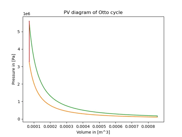
> By using the plot command the state points, volume arrays and pressure arrays are plotted to get the PV diagram of the otto cycle.

Result of the program

> The acquired plot is as shown below

> The thermal efficiency of the engine is

> For the given input parameters of an engine the thermal efficiency is calculated as 62%.

> If the compression ratio is changed then we can acquire different PV diagram acoordingly, with change in vlaues of the state points.

> The efficiency of the engine will aslo change accordingly.