Week 3 - Solving second order ODEs

AIM

To solve second order ordinary differential equation using MATLAB.

GOVERNING EQUATIONS

Where,

g = gravity in m/s2,

L = length of the pendulum in m,

m = mass of the ball in kg,

b=damping coefficient.

OBJECTIVE

1. Write a program in Matlab\Octave that will simulate the pendulum motion.
2. To solve second order ODE with graph.

THEORY

Ordinary Differential Equation: In mathematics, an ordinary differential equation (ODE) is a differential equation containing one or more functions of one independent variable and the derivatives of those functions. In Engineering, ODE is used to describe the transient behavior of a system. A simple example is a pendulum

Simple Pendulum: A simple pendulum can be described as a device where its point mass is attached to a light inextensible string and suspended from a fixed support. The vertical line passing through the fixed support is the mean position of a simple pendulum.

PROGRAM

clear all
close all
clc

% Inputs 
b = 0.05;
g = 9.81;
l = 1;
m = 1;

% Initial angular displacement and angular velocity
theta_0 = [0;3];

% Time span
t_span = linspace(0,20,500);

% Solving ODE
[t,results] = ode45(@(t,theta)ode_fun(t,theta,b,g,l,m),t_span,theta_0);


% Plotting the graph between angular displacement vs time and angular
% velocity vs time
figure(1)

plot(t,results(:,1))

hold on
plot(t,results(:,2))
ylabel('plot')
xlabel('Time')
legend('Angular Displacement','Angular Velocity')


% Animation for simple pendulum
figure(2)

% Fixed Points
x0 = 0;
y0 = 0;
ct = 1;

displacement = results(:,1);
velocity = results(:,2);



for i = 1:length(displacement)
    
    % Coordinates
    x1 = l - l*sin(displacement(i));
    y1 = l - l*cos(displacement(i));
    
    
    % String of pendulum
    plot([1 x1],[1 y1],[x1 x1],[y1 y1],'linewidth',3,'color','r')
    
    % Base bar for pendulum to oscillate
    hold on
    plot([-1 3],[1 1],'color','k','linewidth',7)
    hold off
    
    % Ball that oscillates at the one end of string 
    hold on 
    plot(x1,y1,'O','markers',15,'Markerfacecolor','g')
    hold off
    
    grid on
    
    axis([-1 4 -1 3])
    title('Motion of Pendulum using MATLAB')
    
    % Collecting frames for making animation
    M(ct)=getframe(gcf);
    ct = ct + 1;
end

% To make a movie of collected frames
movie(M)

% saving the file in avi format
videofile = VideoWriter('pendulum.avi','Uncompressed AVI');

% Writing the movie in videofile created
open(videofile)
writeVideo(videofile,M)
close(videofile)

Code function of ode45 for main program

function[dtheta_dt] = ode_fun(t,theta,b,g,l,m)
theta1 = theta(1);
theta2 = theta(2);
dtheta1_dt =theta2;
dtheta2_dt = (-b/m)*theta2 - (g/l)*sin(theta1);
dtheta_dt = [dtheta1_dt;dtheta2_dt];
end

EXPLANATION

1. Initial data are given such as, L=1 metre, m=1 kg, b=0.05 and g=9.81 m/s².
2. Motion is simulated for 20 seconds of time span using the MATLAB command linspace.
3. Initial angular displacement and velocity is provided as the input data and the inbuilt solved function ode45 is called for solving the differential equation.
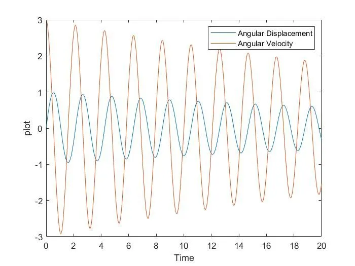
4. Graph is plotted using the plot command for angular displacement and velocity vs time.
5. Animation video of pendulum is created making the fixed coordinates as x0 and y0 and x1, y1 are the other coordinates.
6. Marker command is used to create the bob of the pendulum.
7. videoWrite command is used to create the video file.

RESUlTS

1. Graph for Angular Displacement vs Time and Angular Velocity vs Time is plotted.
   

2. The link for the animation video: https://youtu.be/0JW61MEQHOk

CONCLUSION

1. Animation video of simple pendulum is created.
2. Graph for angular displacement vs time and angular velocity vs time is also plotted.