Project 2 - Rankine cycle Simulator

AIM

Create a Rankine Cycle Simulator using MATLAB/OCTAVE.

THEORY

The Rankine cycle is an idealized thermodynamic cycle describing the process by which certain heat engines, such as steam turbines or reciprocating steam engines, allow mechanical work to be extracted from a fluid as it moves between a heat source and heat sink.

Heat energy is supplied to the system via a boiler where the working fluid (typically water) is converted to a high-pressure gaseous state (steam) in order to turn a turbine. After passing over the turbine the fluid is allowed to condense back into a liquid state as waste heat energy is rejected before being returned to boiler, completing the cycle.

In a Rankine cycle, high-pressure liquid water enters a boiler where it is heated to saturation temperature, vaporized, and superheated. The superheated steam is fed to a turbine, where it expands and generates mechanical work.

Components of Rankine Cycle:

1. Turbine
2. Condenser
3. Pump
4. Boiler

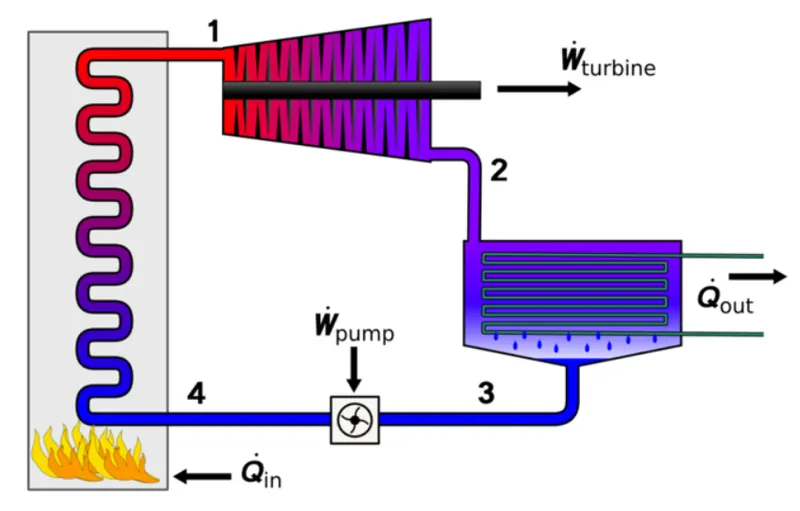
Processes in Rankine Cycle:

• Process 1-2 is Isentropic Expansion in the Turbine
• Process 2-3 is Constant Pressure Heat Rejection by the Condenser
• Process 3-4 is Isentropic Compression in the Pump and
• Process 4-1 is Constant Pressure Heat Addition by the Boiler.

GOVERNING EQUATIONS

• Thermal efficiency is the ratio of the net-work output to the heat input.

η_thermal = W_net/Q_s

• Back work ratio is the ratio of compressor work to turbine work.

BWR = W_P/W_T

• Specific Steam Consumption is defined as the steam consumed by a locomotive's cylinders per unit output of power.

SSC = 3600/W_net

Where,

W_net = W_T-W_P

W_T = Work done by the steam on turbine

W_P = Work done by the pump

Q_s = Heat supplied to the boiler

Q_r = Heat rejected by the condenser

OBJECTIVE

• Calculate the state points of the Rankine Cycle based on user inputs.
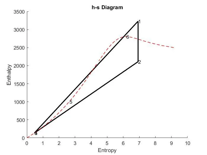
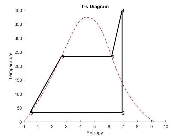
• Plot the corresponding T-s and h-s plots for the given set of inputs.
• Calculate net-work output and back work ratio.

PROGRAM

MATLAB code:

clear all
close all
clc

% Displaying process description
fprintf('\n RANKINE CYCLE SIMULATOR')
fprintf('\n\nProcess 1-2 is Isentropic Expansion in the Turbine')
fprintf('\nProcess 2-3 is Constant Pressure Heat Rejection by the Condenser')
fprintf('\nProcess 3-4 is Isentropic Compression in the Pump')
fprintf('\nProcess 4-1 is Constant Pressure Heat Addition by the Boiler\n')

% Collecting user inputs
p1 = input('\nEnter the Pressure at the Turbine Inlet(in bar) : ');
t1 = input('\nEnter the Temperature at the Turbine Inlet(in degree celcius) : ');
p2 = input('\nEnter the Pressure at the Condenser(in bar) : ');

% Finding state variables with the help of XSteam data 
s1 = XSteam('s_pT',p1,t1);       % Specific entropy at state 1 as a function of pressure and temperature
h1 = XSteam('h_pT',p1,t1);       % Enthalpy at state 1 as a function of pressure and temperature

t3 = XSteam('Tsat_p',p2);        % Temperature at state 3 which is the saturated temperature corresponding to p2
t2 = t3;
p3 = p2;
hf2 = XSteam('hL_p',p2);         
hg2 = XSteam('hV_p',p2);
s2 = s1;
sf2 = XSteam('sL_p',p2);
sg2 = XSteam('sV_p',p2);
x2 = (s2-sf2)/(sg2-sf2);         % Calculating dryness fraction from entropy : s2 = sf2 + x2*(sg2 - sf2)
h2 = hf2 + x2*(hg2 - hf2);       % Calculationg enthalpy at state 2

s3 = sf2;
h3 = hf2;
v3 = XSteam('vL_p',p2);
Wp = v3*(p1-p2)*100;             % Calculating workdone by the pump

p4 = p1;
s4 = s3;
cp4 = XSteam('Cp_ps',p1,s4);     % Specific heat at constant pressure at state 4 as a function of pressure and entropy 
cv4 = XSteam('Cv_ps',p1,s4);     % Specific heat at constant volume at state 4 as a function of pressure and entropy 
gamma = cp4/cv4;               
o = (gamma-1)/gamma;
t4 = t3*((p4/p3)^o);             % t4/t3 = (p4/p3)^[(gamma-1)/gamma]
h4 = Wp + h3;                    % Calculating enthalpy at state 4

Wt = h1-h2;                      % Calculating the workdone by the steam on turbine
Wnet = Wt - Wp;                  % Calculating net work output
Qs = h1 - h4;                    % Calculating heat supplied on the boiler
Qr = h2 - h3;                    % Calculating heat rejected by the condenser
ntherm = (Wnet/Qs)*100;          % Finding thermal efficiency
ssc = 3600/Wnet;                 % Finding Specific steam consumption
bwr = Wp/Wt;                     % Finding back work ratio

% Printing the outputs
% State 1 
fprintf('\n\nAt state point 1:')
fprintf('\nP1 is : %f Bar',p1)
fprintf('\nT1 is : %f Degree celcius',t1)
fprintf('\nS1 is : %f kJ/kgK',s1)
fprintf('\nH1 is : %f kJ/kg',h1)

% State 2
fprintf('\n\nAt state point 2:')
fprintf('\nP2 is : %f Bar',p2)
fprintf('\nT2 is : %f Degree celcius',t2)
fprintf('\nS2 is : %f kJ/kgK',s2)
fprintf('\nH2 is : %f kJ/kg',h2)
fprintf('\nX2 is : %f ',x2)

% State 3
fprintf('\n\nAt state point 3:')
fprintf('\nP3 is : %f Bar',p3)
fprintf('\nT3 is : %f Degree celcius',t3)
fprintf('\nS3 is : %f kJ/kgK',s3)
fprintf('\nH3 is : %f kJ/kg',h3)

% State 4
fprintf('\n\nAt state point 4:')
fprintf('\nP4 is : %f Bar',p4)
fprintf('\nT4 is : %f Degree celcius',t4)
fprintf('\nS4 is : %f kJ/kgK',s4)
fprintf('\nH4 is : %f kJ/kg',h4)

% State 5 and 6 for plotting
p5 = p1;
t5 = XSteam('Tsat_p',p1);             % Temperature at state 5 is the saturated temperature as a function of pressure  
h5 = XSteam('hL_p',p1);               % Enthalpy at state 5 as a function of pressure at liquid state
s5 = XSteam('sL_p',p1);               % Entropy at state 5 as a function of pressure at liquid state

t6 = t5;
p6 = XSteam('Psat_T',t6);             % Pressure at state 6 is the saturated pressure as a function of temperature
h6 = XSteam('hV_T',t6);               % Enthalpy at state 6 as a function of temperature at vapour state
s6 = XSteam('sV_T',t6);               % Entropy at state 6 as a function of temperature at vapour state


% Printing the outputs
fprintf('\n\nWork done by the steam Wt : %f kJ/kg',Wt)
fprintf('\nWork done by the pump Wp : %f kJ/kg',Wp)
fprintf('\nNet work output Wnet : %f kJ/kg',Wnet)
fprintf('\nThermal efficiency of the Rankine cycle : %f ',ntherm)
fprintf('\nSpecific Steam Consumption of the Rankine cycle : %f kg/kWh',ssc)
fprintf('\nBack Work Ratio of the Rankine cycle : %f \n',bwr)


% Plotting
t_curve = linspace(0,500,1000);
for i = 1:length(t_curve)
    s_L(i) = XSteam('sL_T',t_curve(i));     % Saturated liquid entropy
    s_V(i) = XSteam('sV_T',t_curve(i));     % Saturated vapour entropy
    h_L(i) = XSteam('hL_T',t_curve(i));     % Saturated liquid enthalpy
    h_V(i) = XSteam('hV_T',t_curve(i));     % Saturated vapour enthalpy
end

figure(1)
hold on
plot([s1 s2 s3 s4 s5 s6 s1],[t1 t2 t3 t4 t5 t6 t1],'color','k','linewidth',2)
plot(s_L,t_curve,'color','r','linestyle','--','linewidth',1)
plot(s_V,t_curve,'color','r','linestyle','--','linewidth',1)
text(s1,t1,'1')
text(s2,t2,'2')
text(s3,t3,'3')
text(s4,t4,'4')
text(s5,t5,'5')
text(s6,t6,'6')
xlabel('Entropy')
ylabel('Temperature')
title('T-s Diagram')


figure(2)
hold on
plot([s1 s2 s3 s4 s1],[h1 h2 h3 h4 h1],'color','k','linewidth',2)
plot(s_L,h_L,'color','r','linestyle','--','linewidth',1)
plot(s_V,h_V,'color','r','linestyle','--','linewidth',1)
text(s1,h1,'1')
text(s2,h2,'2')
text(s3,h3,'3')
text(s4,h4,'4')
text(s5,h5,'5')
text(s6,h6,'6')
xlabel('Entropy')
ylabel('Enthalpy')
title('h-s Diagram')

Explanation of the code

1. Program begins with basic commands like clear all, close all and clc which clears the workspace, closes all the plots and clear the command window respectively.
2. Next step is to print the processes involved in a Rankine cycle for the user to get a clear-cut idea of Rankine cycle. To print the statements fprintf command is used.
3. Using input command, the required inputs are collected from the user end and are saved in different variables.
4. From the input data available, entropy, enthalpy, temperature, pressure and all other parameters which all are required is collected. For this, XSteam data table is used which is provided as an attachment.
5. Pressure, temperature, enthalpy and entropy for all the state variables are extracted as a function of the dependent variable in XSteam file.
6. Work done by the pump, work done by the steam on turbine, net work output, heat supplied to the boiler, heat rejected from the condenser, thermal efficiency, specific steam consumption and back work ratio are all identified from the known data by applying the direct formula for the required.
7. Now the outputs are printed out in an ordered manner starting from state one to state four. Pressure, temperature, entropy and enthalpy of all these four points are printed in sequence manner.
8. Work done by the steam on turbine, work done by the pump, net work output, thermal efficiency, specific steam consumption and back work ratio are all printed with the help of fprintf command
9. Temperature is divided into 1000 points to find saturated entropy and enthalpy at each temperature for both liquid as well as vapour state to draw saturated curve.
10. Plotting is done with labelling on both x and y axis along with the titles are also provided. Thus h-s and T-s diagram are plotted with proper labelling.

RESULTS

Required Inputs:

Turbine Inlet temperature = 400° C

Turbine Inlet Pressure = 30 bars

Turbine Outlet Pressure = 0.05 bars = Condenser Inlet Pressure

Outputs from command Window:

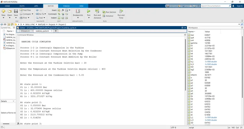
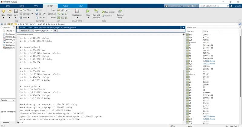
From above, we can see that

1. Work done by the steam Wt : 1120.862815 kJ/kg
2. Work done by the pump Wp : 3.010937 kJ/kg
3. Net-work output Wnet : 1117.851878 kJ/kg
4. Thermal efficiency of the Rankine cycle : 36.167131
5. Specific Steam Consumption of the Rankine cycle : 3.220462 kg/kWh
6. Back Work Ratio of the Rankine cycle : 0.002686

Plots Obtained:

1. H - S Diagram

2. T - S Diagram

CONCLUSION

• MATLAB code for Rankine cycle simulator is done for the user inputs.
• H-S diagram and T-S diagram for the user inputs is plotted.
• Net-work output for the Rankine cycle is calculated and it is equal to 1117.851878 kJ/kg.
• Back work ratio for the Rankine cycle is calculated and is equal to 0.002686.