Week 4.1 - Genetic Algorithm
AIM
To optimize the stalagmite function and to find global maxima of the function.
THEORY
A genetic algorithm (GA) is a method for solving both constrained and unconstrained optimization problems based on a natural selection process that mimics biological evolution. The algorithm repeatedly modifies a population of individual solutions. At each step, the genetic algorithm randomly selects individuals from the current population and uses them as parents to produce children for the next generation. Over successive generations, the population "evolves" toward an optimal solution.
In MATLAB, ga - Find minimum of function using genetic algorithm.
It is frequently used to find optimal or near optimal solutions to difficult problems. Optimization refers to the process of making something better. It is a study that deals with how to minimize or maximize a particular function which depends on multiple input parameters.
In ga, we have a pool or a population of possible solutions to the given problem. This solution undergoes recombination and mutation, producing new children and the repeated over various generations.
Population is a subset of all the possible solutions to the given problem.
Population Options:
Population options let you specify the parameters of the population that the genetic algorithm uses.
- PopulationType: specifies the type of input to the fitness function.
- PopulationSize: specifies how many individuals there are in each generation. With a large population size, the genetic algorithm searches for the solution space more thoroughly, thereby reducing the chance that the algorithm returns a local minimum that is not a global minimum. However, a large population size also causes the algorithm to run more slowly. The default is '50 when numberOfVariables <= 5, else 200'.
Each individual is assigned a fitness value and the fitter individuals are given a higher chance to mate and yield more fitter individuals. In this way we keep evolving better individuals or solutions over generations till we reach a stopping criterion.
Stopping Criteria Options
Stopping criteria determine what causes the algorithm to terminate
You can specify the following options:
- MaxGenerations — Specifies the maximum number of iterations for the genetic algorithm to perform.
- MaxTime — Specifies the maximum time in seconds the genetic algorithm runs before stopping, as measured by tic and toc. This limit is enforced after each iteration, so ga can exceed the limit when an iteration takes substantial time.
- FitnessLimit — The algorithm stops if the best fitness value is less than or equal to the value of FitnessLimit.
- MaxStallGenerations — The algorithm stops if the average relative change in the best fitness function value over MaxStallGenerations is less than or equal to FunctionTolerance.
- MaxStallTime — The algorithm stops if there is no improvement in the best fitness value for an interval of time in seconds specified by MaxStallTime, as measured by tic and toc.
- FunctionTolerance — The algorithm stops if the average relative change in the best fitness function value over MaxStallGenerations is less than or equal to FunctionTolerance.
- ConstraintTolerance — The ConstraintTolerance is not used as stopping criterion. It is used to determine the feasibility with respect to nonlinear constraints.
Fitness Function: It is a function which takes the solution as input and produces the suitability of the solution as the output.
Genetic Operators: Alter the genetic composition of the offspring. This includes crossover, mutation, selection etc.
Basic Structure:
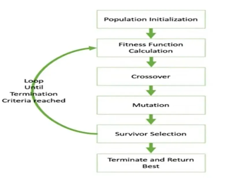
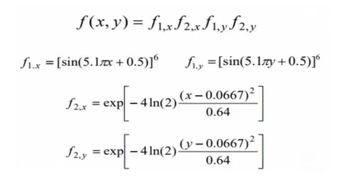
Stalagmite function is a mathematical model that actually helps us to generate local minima and maxima. It is a three-dimensional function.
Syntax for ga is:
- x = ga(fun,nvars,A,b) finds a local minimum x to fun, subject to the linear inequalities A*x ≤ b. ga evaluates the matrix product A*x as if x is transposed (A*x').
- x = ga(fun,nvars,A,b,Aeq,beq) finds a local minimum x to fun, subject to the linear equalities Aeq*x = beq and A*x ≤ b. (Set A = [] and b = [] if no linear inequalities exist.) ga evaluates the matrix product Aeq*x as if x is transposed (Aeq*x').
- x = ga(fun,nvars,A,b,Aeq,beq,lb,ub) defines a set of lower and upper bounds on the design variables, x, so that a solution is found in the range lb ≤ x ≤ ub. (Set Aeq = [] and beq = [] if no linear equalities exist.)
- x = ga(fun,nvars,A,b,Aeq,beq,lb,ub,nonlcon) subjects the minimization to the constraints defined in nonlcon. The function nonlcon accepts x and returns vectors C and Ceq, representing the nonlinear inequalities and equalities respectively. ga minimizes the fun such that C(x) ≤ 0 and Ceq(x) = 0. (Set lb = [] and ub = [] if no bounds exist.)
- x = ga(fun,nvars,A,b,Aeq,beq,lb,ub,nonlcon,options) minimizes with the default optimization parameters replaced by values in options. (Set nonlcon = [] if no nonlinear constraints exist.) Create options using optimoptions.
- x = ga(fun,nvars,A,b,Aeq,beq,lb,ub,nonlcon,intcon) or x = ga(fun,nvars,A,b,Aeq,beq,lb,ub,nonlcon,intcon,options) requires that the variables listed in intcon take integer values. When there are integer constraints, ga does not accept nonlinear equality constraints, only nonlinear inequality constraints.
PROCEDURE
- Initially the program starts with the basic commands such as clear all, close all and clc.
- Search space is defined in the variables x and y using the linspace command, and thus a one-dimensional array is formed.
- A three-dimensional mesh grid xx and yy is created using the command meshgrid. This can be used to evaluate our stalagmite function of two variables.
- Next, two for loops are called which gives us the data for the plot of 3D. Now the values in the different matrices created can be put as an input into the function and thus we will get the value of stalagmite function at various values of x and y.
- The total number of times the ga needs to run is defined using the num_cases and with the help of for loop ga is made to run for each iteration and the value is stored in an array.
- ga command is called for finding the global maxima. Generally, ga gives us only the minima, but our aim is to calculate the global maxima. For that we had changed the equations in the stalagmite formula by assigning a negative value for the final result. Governing equation
- The first study concerns with the unbounded inputs provided for calculating the value of global maxima.
- Study two was concerned with the bounded inputs provided for calculating the value of global maxima. So, the syntax of ga is changed in the second study by providing upper and lower bounds.
- Third study concerns with bounded inputs provided but with varied population size for better optimization in order to calculate the value of global maxima. So, corresponding changes as provided for the ga syntax.
- Using tic and toc commands we can identify how long the program takes to complete the study.
- To visualize the function plot clearly, surfc command is used.
- Shading interp command is used, so the graph obtained will be without any grids.
PROGRAM
MATLAB code to optimize the stalagmite function and for finding global maxima is:
The main program with separate explanation:
clear all
close all
clc

% defining our search space
x = linspace(0,0.6,150);
y = linspace(0,0.6,150);

% creating a 3 dimensional mesh
[xx yy] = meshgrid(x,y);

% evaluating the stalagmite function
for i = 1 : length(xx)
    for j = 1 : length(yy)
        input_vector(1) = xx(i,j);
        input_vector(2) = yy(i,j);
        f(i,j) = stalagmite_fun(input_vector);
    end
end

num_case = 50;  % By assigning num_cases, it will make the 'ga' to run 50 times inside the upcoming for loop
Study 1: Here, the algorithm is studied by not defining the limits. The ga does not run within a particular search space as we haven’t defined the bounds.
% Study 1 statistical behaviour without any bounds
tic
for i = 1:num_case
    [inputs , fopt(i)] = ga(@stalagmite_fun,2);
    xopt(i) = inputs(1);
    yopt(i) = inputs(2);
end
study1_time = toc % To know how long it takes to complete the study

% Plotting the graphs
figure(1)
subplot(2,1,1) % Using subplot command we can represent multiple plots in single graph
hold on
surfc(x,y,-f) % Surface plot to visualize the function
shading interp % This command will helps to represent the graph without grids
plot3(xopt,yopt,-fopt,'marker','o','markersize',5,'markerfacecolor','r') % 3D plotting which heps to visualise how the algorithm is performing
title('Unbounded inputs')

subplot(2,1,2)
plot(-fopt) % Optimum value is plotted that the function is predicting
xlabel('Iterations')
ylabel('Function maximum')
Study 2: Here, the lower and upper bounds are defined so as to know the boundaries within the global maxima lies i.e., here we define a definite space within which the global maxima is to be found.
% Study 2 - statistical behaviour with upper and lower bounds
tic
for i = 1:num_case
    [inputs , fopt(i)] = ga(@stalagmite_fun,2,[],[],[],[],[0;0],[0.6;0.6]); % upper and lower bounds are provided as 0 to 0.6
    xopt(i) = inputs(1);
    yopt(i) = inputs(2);
end
study2_time = toc

% Plotting
figure(2)
subplot(2,1,1)
hold on
surfc(x,y,-f)
shading interp
plot3(xopt,yopt,-fopt,'marker','o','markersize',5,'markerfacecolor','r')
title('Bounded inputs')

subplot(2,1,2)
plot(-fopt)
xlabel('Iterations')
ylabel('Function maximum')
Study 3: Here, we are defining population size along with the lower and upper bounds. The population size is increased so as to converge to a better optimal solution of global maxima.
%study 3 - Increasing GA iterations
options = optimoptions('ga');
options = optimoptions(options,'Populationsize',170);

tic
for i = 1:num_case
    [inputs , fopt(i)] = ga(@stalagmite_fun,2,[],[],[],[],[0;0],[0.6;0.6],[],[],options); % Upper and lower bounds are provided along with increased populaion size
    xopt(i) = inputs(1);
    yopt(i) = inputs(2);
end
study3_time = toc

% Plotting
figure(3)
subplot(2,1,1)
hold on
surfc(x,y,-f)
shading interp
plot3(xopt,yopt,-fopt,'marker','o','markersize',5,'markerfacecolor','r')
title('Bounded inputs with modified population size')

subplot(2,1,2)
plot(-fopt)
xlabel('Iterations')
ylabel('Function maximum')
The main program as a whole:
clear all
close all
clc

% defining our search space
x = linspace(0,0.6,150);
y = linspace(0,0.6,150);

% creating a 3 dimensional mesh
[xx yy] = meshgrid(x,y);

% evaluating the stalagmite function
for i = 1 : length(xx)
    for j = 1 : length(yy)
        input_vector(1) = xx(i,j);
        input_vector(2) = yy(i,j);
        f(i,j) = stalagmite_fun(input_vector);
    end
end


num_case = 50;  % By assigning num_cases, it will make the 'ga' to run 50 times inside the upcoming for loop


% Study 1 statistical behaviour without any bounds
tic
for i = 1:num_case
    [inputs , fopt(i)] = ga(@stalagmite_fun,2);
    xopt(i) = inputs(1);
    yopt(i) = inputs(2);
end
study1_time = toc % To know how long it takes to complete the study

% Plotting the graphs
figure(1)
subplot(2,1,1) % Using subplot command we can represent multiple plots in single graph
hold on
surfc(x,y,-f) % Surface plot to visualize the function
shading interp % This command will helps to represent the graph without grids
plot3(xopt,yopt,-fopt,'marker','o','markersize',5,'markerfacecolor','r') % 3D plotting which heps to visualise how the algorithm is performing
title('Unbounded inputs')

subplot(2,1,2)
plot(-fopt) % Optimum value is plotted that the function is predicting
xlabel('Iterations')
ylabel('Function maximum')


% Study 2 - statistical behaviour with upper and lower bounds
tic
for i = 1:num_case
    [inputs , fopt(i)] = ga(@stalagmite_fun,2,[],[],[],[],[0;0],[0.6;0.6]); % upper and lower bounds are provided as 0 to 0.6
    xopt(i) = inputs(1);
    yopt(i) = inputs(2);
end
study2_time = toc

% Plotting
figure(2)
subplot(2,1,1)
hold on
surfc(x,y,-f)
shading interp
plot3(xopt,yopt,-fopt,'marker','o','markersize',5,'markerfacecolor','r')
title('Bounded inputs')

subplot(2,1,2)
plot(-fopt)
xlabel('Iterations')
ylabel('Function maximum')


%study 3 - Increasing GA iterations
options = optimoptions('ga');
options = optimoptions(options,'Populationsize',170);

tic
for i = 1:num_case
    [inputs , fopt(i)] = ga(@stalagmite_fun,2,[],[],[],[],[0;0],[0.6;0.6],[],[],options); % Upper and lower bounds are provided along with increased populaion size
    xopt(i) = inputs(1);
    yopt(i) = inputs(2);
end
study3_time = toc

% Plotting
figure(3)
subplot(2,1,1)
hold on
surfc(x,y,-f)
shading interp
plot3(xopt,yopt,-fopt,'marker','o','markersize',5,'markerfacecolor','r')
title('Bounded inputs with modified population size')

subplot(2,1,2)
plot(-fopt)
xlabel('Iterations')
ylabel('Function maximum')
Stalagmite function program for the main program:
function output = stalagmite_fun(input_vector)
f1x = [sin(5.1*pi*input_vector(1) + 0.5)]^6;
f1y = [sin(5.1*pi*input_vector(2) + 0.5)]^6;
f2x = exp((-4*log(2)*(input_vector(1)-0.0667)^2)/0.64);
f2y = exp((-4*log(2)*(input_vector(2)-0.0667)^2)/0.64);
output = -(f1x*f1y*f2x*f2y);
end
RESULTS
Result 1:
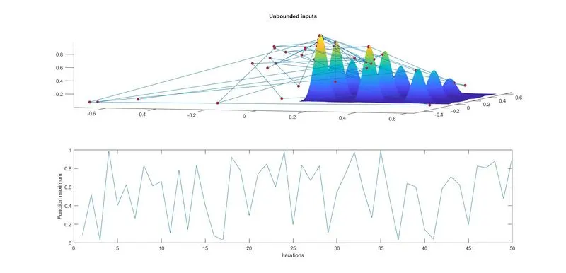
From the figure as shown above, it is clear that the results are not accurate and gives a lot of variation in optimizing the function. It can be observed that the value of Function maximum lies between the interval 0 and 1.
Result 2:
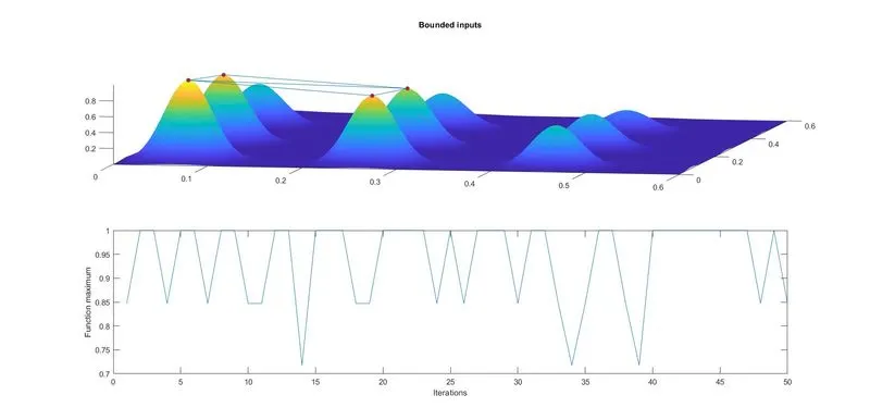
Here, it is clearly seen that, after providing the lower and upper bounds, the variation in the optimum value of the function had reduced. The value of Function maximum here lies between 0.7 and 1.
Result 3:
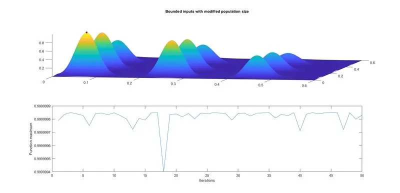
It is clear from the graph that the value of the variation range has changed to a large extent as we had provided population size along with the lower and upper bounds. Here the probability of determining the exact value of global maxima is much more increased and the value comes out to be 0.99999985.
CONCLUSION
The global maxima is calculated by population sizing and the plots are also provided.
It is also observed that the study time increases as boundary conditions and population size is enabled. Thus study 3 took more time to complete and least time for study 1.
REFERENCES
https://in.mathworks.com/help/gads/what-is-the-genetic-algorithm.html
https://en.wikipedia.org/wiki/Genetic_algorithm
https://in.mathworks.com/help/gads/how-the-genetic-algorithm-works.html#f6243