Week 3 - External flow simulation over an Ahmed body.

Introduction to GUI based CFD using ANSYS Fluent

Ahmed Body - Report - WEEK 3

B A Mayur

INTRODUCTION

An ahmed body represents a standard passenger car. It has a blunt rear region to simulate the wake region and the aerodynamics is such that it is sufficient to simulate a flow around the body to validate pressure to be minimized around the front section of the body with respect to the flow direction. This way the velocity components are tangent to the surface with an aesthetic approach. The model was developed to validate CFD codes with experimental data.

AIM

• To obtain the negative coefficient of pressure using vector plot at the wake region after performing a grid independency test
• To obtain the significance of point of separation using information from pressure and velocity contours as well as lift and drag values/charts.

THEORY OF THE PROBLEM

In this report, the problem statement relates to the flow around an ahmed body. The area of concern being around the body, the mesh must be checked and optimized in the proximity rather than the mesh inside the body where flow does not occur. Using SpaceClaim, we can model an overall enclosure for the simulation and an inner enclosure/computational domain to measure physical parameters around the ahmed body.

The volume extract of the ahmed body is taken off using “Suppress for physics” option. Cut-plane option is used for confirmation of no-mesh region within the ahmed body. The faces are named to apply boundary conditions and brought into the ANSYS Fluent environment. A pressure-based solver is used and a grid independence test is made to obtain optimum usage of system specifications and time efficiency for close-to-accurate results. K-e turbulence model is the initial choice for validating results without the use of energy equation as thermal parameters are not required to be specified in this case. Planes, contours and charts are depicted to understand and study the phenomenon that occurs around the body as a result of the simulation.

GOVERNING EQUATIONS AND OTHER SUPPORTING EQUATIONS

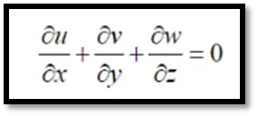
The conservation of mass, momentum and energy equations are used to calculate the problem and validate the analysis.

Conservation of mass equation:

Conservation of momentum equation:

Reynolds Number (Re):

Where ‘ρ’ is the density in kg/m³, ‘v’ is the velocity in m/s, ‘D’ is the diameter of the cylinder in meter and ‘μ’ is the dynamic viscosity of the fluid in N/m².

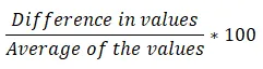
The formula for difference percentage is:

SOLVING AND MODELING APPROACH

The geometry for the computational domain is given in the figure below. The volume dimensions are shown in SolidWorks software after conversion of the geometry file to a step file from SpaceClaim. The length, breadth and height values are roughly measured to be 1m x 0.4m x 0.3m for a cuboid which is modified to form the ahmed body by modeling the front and rear sections for an aerodynamic approach with respect to the flow direction.

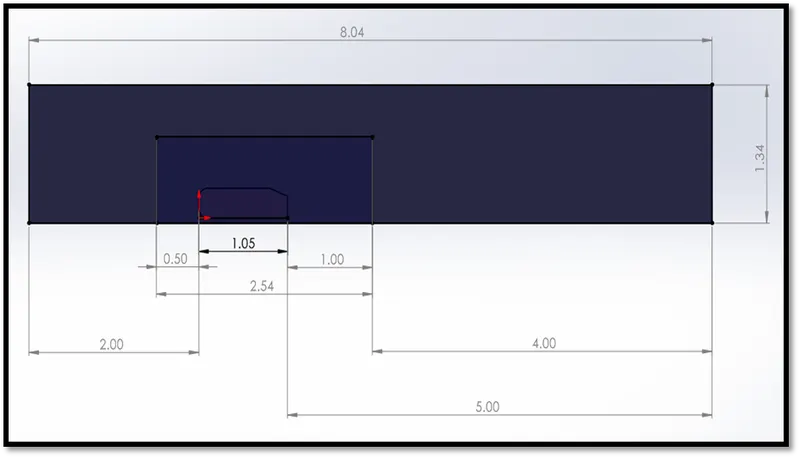
Fig: Dimensions for the simulation model –Front Plane

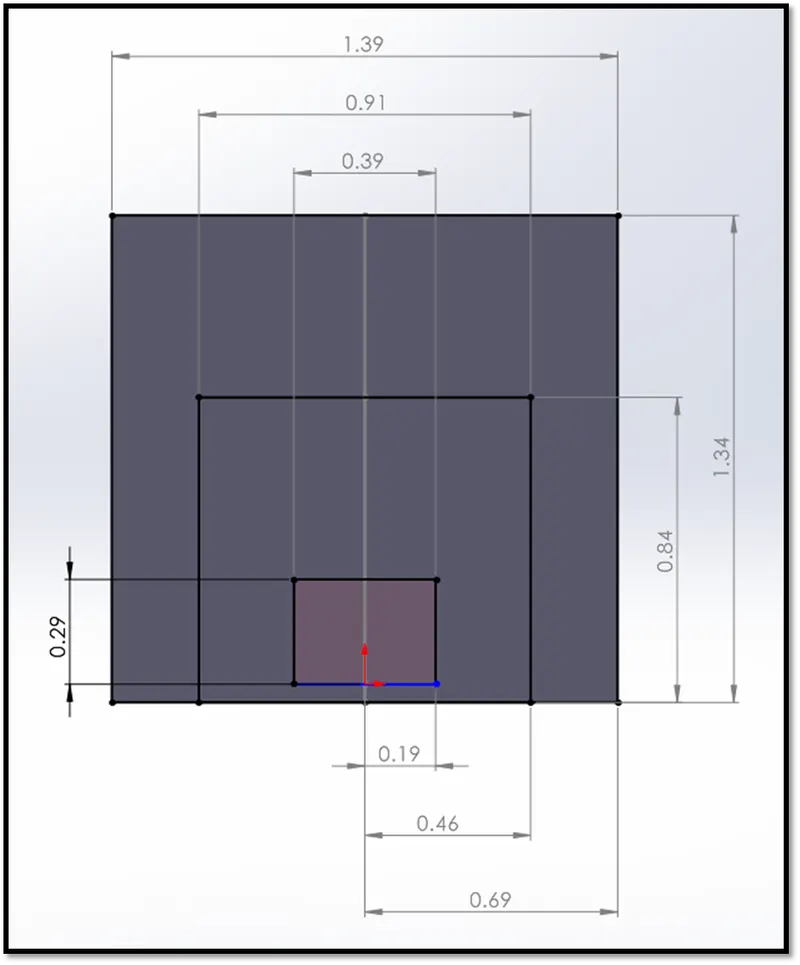
Fig: Dimensions for the simulation model –Right Plane

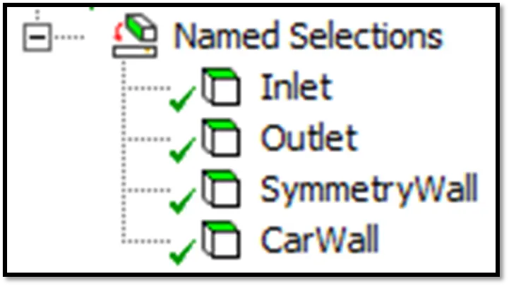
The dimensions are mentioned and a figure is drawn using SpaceClaim in ANSYS Workbench to create enclosures. They are varied with respect to the origin located below the front section close to the ahmed body as shown in the figure. With respect to this origin, the inlet section is measured as 2m. The distance between the rear section of the ahmed body and the outer computational domain is 5m. The area or the enclosure which is enveloped by the outer enclosure is referred to as the inner computational domain or the refined mesh region to capture the flow effects accurately. This enclosure is refined as it is close to the body to simulate the flow effects. It is ensured that the mesh within the ahmed body is subtracted or taken off as flow does not take place here. Rather the flow around the body is to be simulated which being the reason for local refinement. Both the outer and inner enclosures can be considered to simulate the effects of a wind tunnel for the flow domain. Named selections are chosen to apply boundary conditions for outer enclosure inlet, outlet, symmetry wall and car wall (ahmed body wall). To ensure that the mesh is uniform between enclosures, the interference tool is used to fix the problem. This makes a shared topology for mesh intersections between enclosures to avoid grid shocks against inaccurate results.

A base mesh is first created for the geometry. The mesh data is generated for hexahedral mesh (high quality mesh) and the multi-zone mesh method enables to create hexahedral mesh wherever possible. The mesh data maximum size is altered (approx. 100 mm) to get an evenly sized mesh in the outer regions and a grid dependency test is performed considering the inner enclosure (element size = 100 mm , 50 mm and 35 mm) where a more refined mesh generation than outer enclosure is sensible. Similarly, the ahmed body can have a mesh element size around 10mm or even lesser based on the computational power, but in this case only the overall mesh element size values are mentioned and not individually specified for car wall and enclosures.

Each cell has it’s cell centers at different locations. We want to create a set of cells that follow the walls or shape of the surface quite closely for effective boundary conditions applied to walls. Here, the inflation layer option is chosen and a total thickness is mentioned for the ahmed body. This will constrain the mesh in the right direction close to the walls to apply the boundary conditions effectively. These are the parameters to effectively conduct a grid independency test. Since the flow around the “passenger car” is of our interest, it is recommended and implied logically that the mesh data of the ahmed body and inner enclosure be varied with respect to the base/default mesh.

Below is an image of the model having a base mesh generated on which the simulation can be performed for a grid independency test.

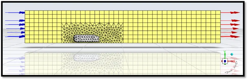
Fig: Ahmed Body Base Mesh Setup

The mesh size of the model is set to 100 mm element size. The inflation layers are created with first layer height of 1.48771324174329E-02 mm, a growth rate of 1.1 for a maximum of 40 layers to enhance refinement near the walls of the passenger car. We must make sure that the geometry on top of which we want to simulate the flow are captured perfectly. This calls for the need of a perfect body fitted mesh. The mesh for Case ‘B’, i) has 12234 nodes, 23436 cells and 58173 faces.

This means that for every 110%, the mesh elements vary in distance away from the cylinder edge.

In this report, ANSYS FLUENT 2020 R1 is used to capture the results by performing the simulation. The solver type is a pressure based to solve the steady flow problem.

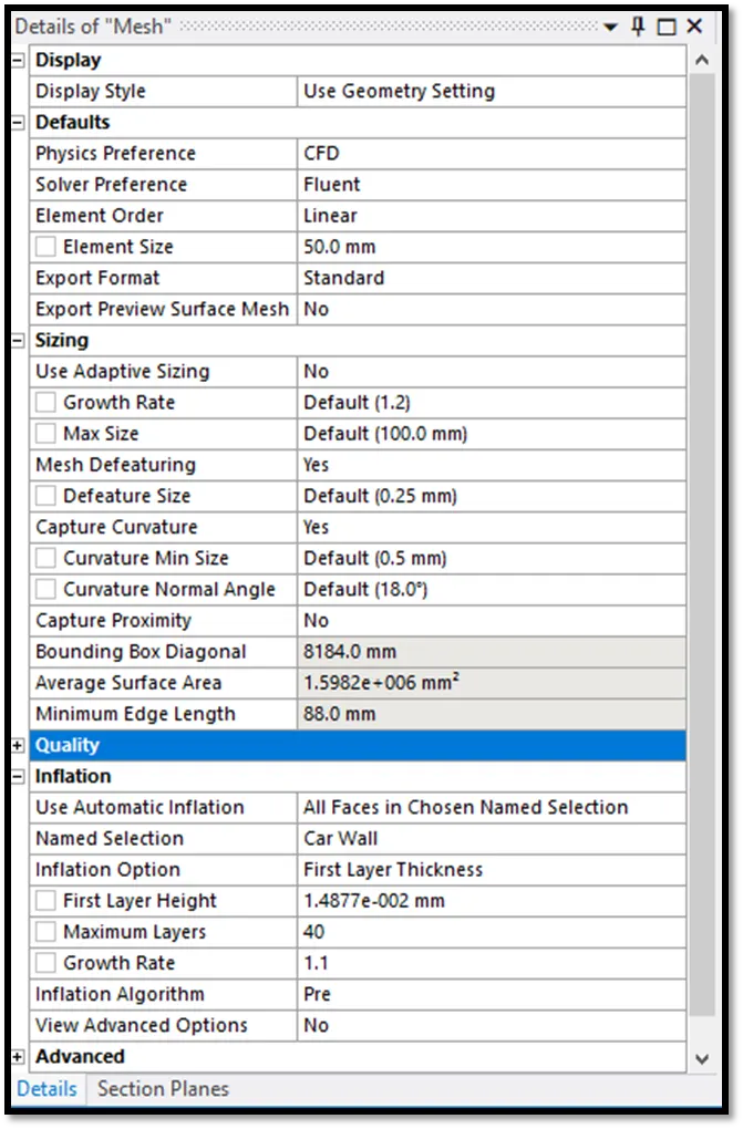
Fig: Case ‘B’ ii) Mesh Details

For Case ‘B’, ii), the mesh details are given in the above image. A maximum element size of 50 mm is used making the case finer than i). For Case ‘B’, iii), a relatively higher refined mesh is generated with an element size set as 35 mm with same inflation layer details.

The simulations are divided into two cases ‘A’ and ‘B’. Case ‘A’ comprises of i) and ii) sub-cases for k-e and k-w models respectively. Case ‘B’ consists of sub-cases i), ii) and iii) for the grid independency tests.

Mesh Details

Case ‘A’
	Element Size	Cells	Faces	Nodes
i) k-e model	50 mm	147548	370844	85558
ii) k-w model	50 mm	246413	617808	135342
Case ‘B’ – Laminar turbulence models for Grid Independency Test
i) Base Mesh	100 mm	23436	58173	12234
ii) Refined mesh	50 mm	246413	617808	135342
iii) More refined	35 mm	411500	1056536	252301

The table above shows the values for number of cells, nodes and faces for the specified overall mesh element size for both cases, ‘A’ and ‘B’.

TURBULENCE MODELS

The model specifies options for control of the flow. Here the laminar flow option is selected for the grid independency test which specifies that the flow is not turbulent in nature and the flow has a low Reynolds number around 100 by varying the velocity. A pressure based solver is used to proceed with a steady state approach for a mach number below 0.3.

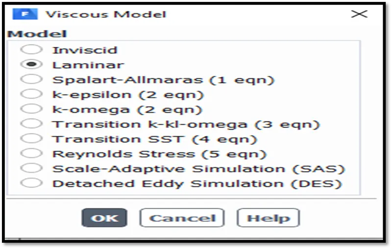
By varying the velocity, the change in the Reynolds number can be optimized, here the velocity is set to 25m/s for all cases. A user defined type fluid or a “customized fluid” is set towards the optimization of obtaining flow effects around the body. The density is 1.225kg/m³ and thus the chosen turbulence model (laminar viscous model) will be sufficient for the simulation to obtain the results within an expected margin of error for the streamlined flow to obtain the grid independency test results.

PRE-PROCESSING AND SOLVER SETTINGS

The fluid domain is defined as air and the boundary of the solid-fluid interference is defined as wall. The energy equation is usually turned on to facilitate setting the temperature parameters of the system but here in this case, it is not required as the flow does not need setting up of thermal properties. The velocity at inlet is set to 25m/s. The gauge pressure is equal to 0 as this is the atmospheric pressure (1atm) and the gauge reads zero unless triggered. The boundary conditions for the inlets are velocity type inlets and pressure based outlets with no specific values set by the user. The backflow pressure specification at outlet is set to total pressure and is solved by the solver after initialization.

Below are descriptive images to show the boundary conditions and solver settings to proceed with simulation using a steady state solver for the k-e turbulence model.

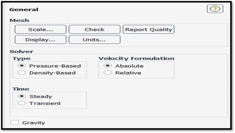
Pressure based solver and a steady state approach is chosen for the simulation.

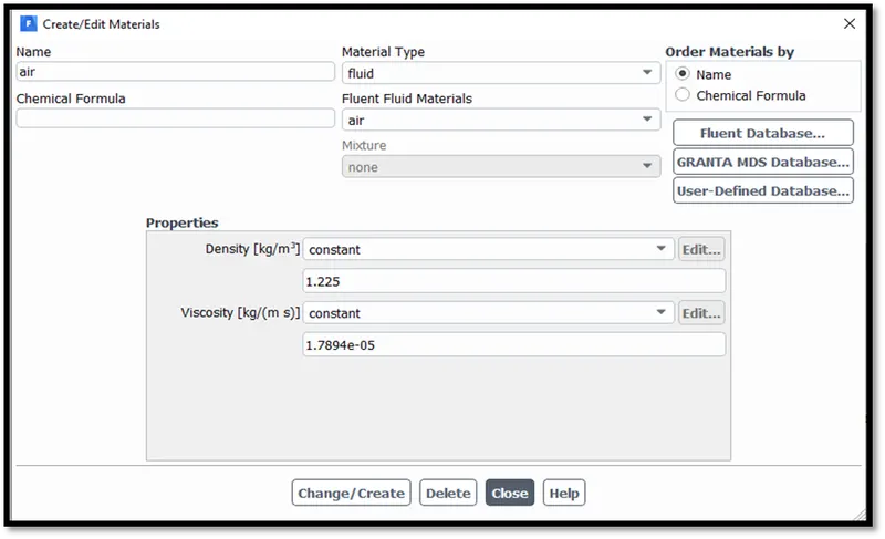
The density of the fluid (air) is set to 1.225kg/m³ with a viscosity of 0.05kg/ms.

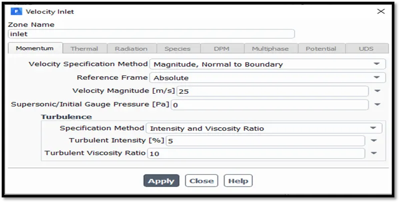
The velocity of the fluid at inlet is set to 25m/s.

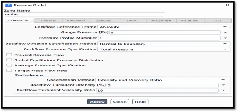
The gauge pressure is mentioned as 0 i.e., 1 atm pressure.

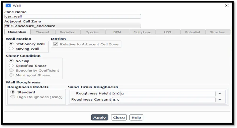
A no slip condition is specified for the flow around the car wall edges. This helps to consider the friction effects and creating a velocity profile near the wall. At the wall, the velocity is zero. Due to adhesion or intermolecular forces between solid-fluid and fluid-fluid molecular interactions, the molecular attractive forces of the viscous sub-layer have a tendency to resist the movement or rate of change of time of the buffer layer above the wall. This in turn has a relatively lower force being exerted by the layers as progressed away from the wall, thus creating a velocity profile being caused by the viscosity.

RESULTS

CASE ‘A’ – k-e and k-w Turbulence Models

1. The k-e turbulence model

In this section, the k-e turbulence model solves two transport equations (PDEs) to encounter the effects more accurately at regions away from the car wall. Hence to capture the flow effects near the car wall, a y+ value of 50 is required.

1. The k-w turbulence model

The k-w turbulence model is best used to capture the near wall effects at adverse pressure gradients. Thus a y+ value of only 1 is sufficient to capture the effects near the ahmed body to define the inflation layers.

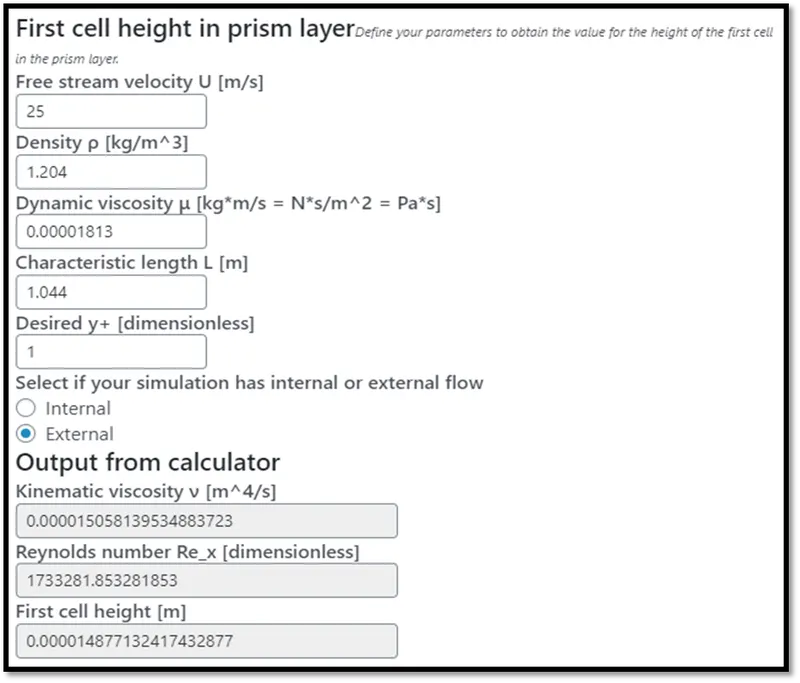
Fig: y+ value for k-w turbulence model is 0.014877 mm

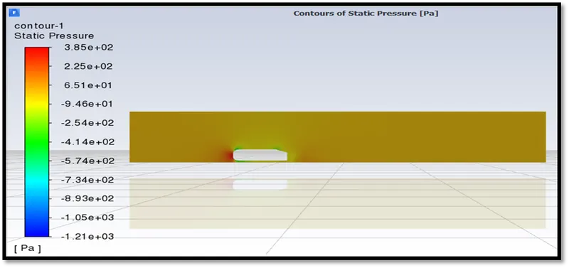
Fig: Pressure contour of k-e model (1)

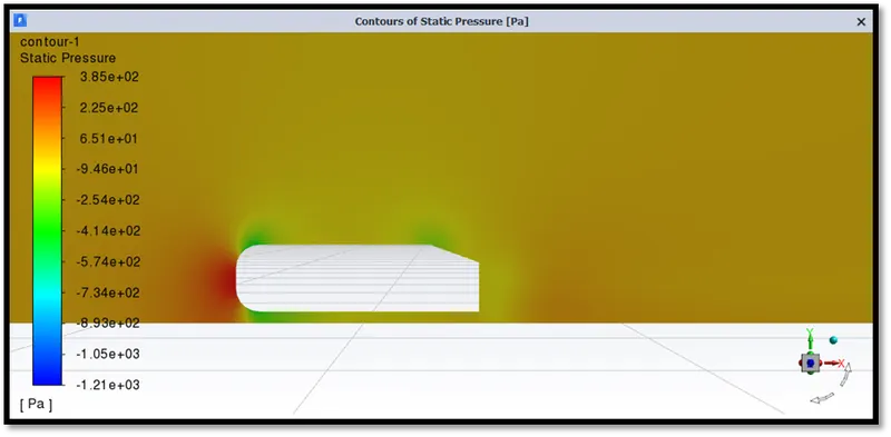
Fig: Pressure contour of k-e model (2)

It is observed that there are stagnation points at the front section of the car wall by looking at the pressure contour and at the rear of the ahmed body with the help of the velocity contour. In this case, both the pressure and velocity are not co-related.

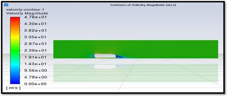
Fig: Velocity contour of k-e model (1)

The stagnation points are formed as kinetic energy is converted to pressure energy, a high pressure region is formed. It can be better depicted as boundary layer is captured by inflation layers and better mesh generation capabilities.

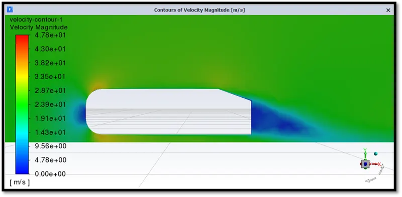
Fig: Velocity contour of k-e model (2)

The contour shows that there are close to zero velocity values obtained at front and rear sections of the car wall. The image below shows the flow separation point as encircled. For a flat plate the velocity is close to zero at all point near the wall. But for a curved surface as in this case of the car wall rear section where the flow separation happens, the velocity gradients tend to change it’s direction as shown in the figure following the image. This is the wake region, where the velocity vectors are close to zero or even negative close to the point of separation, forming the recirculating zone downstream of the flow.

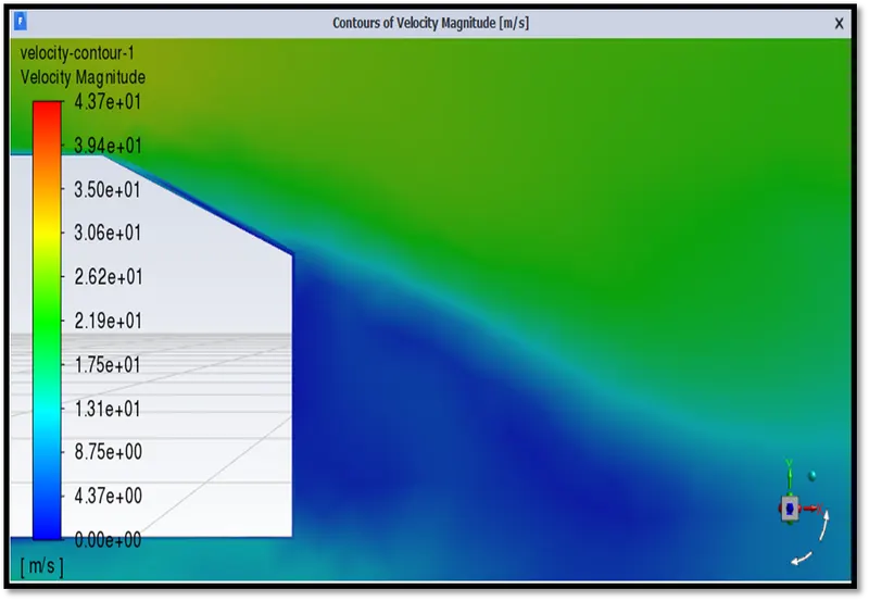
Fig: Velocity contour of k-e model – Flow Separation (2)

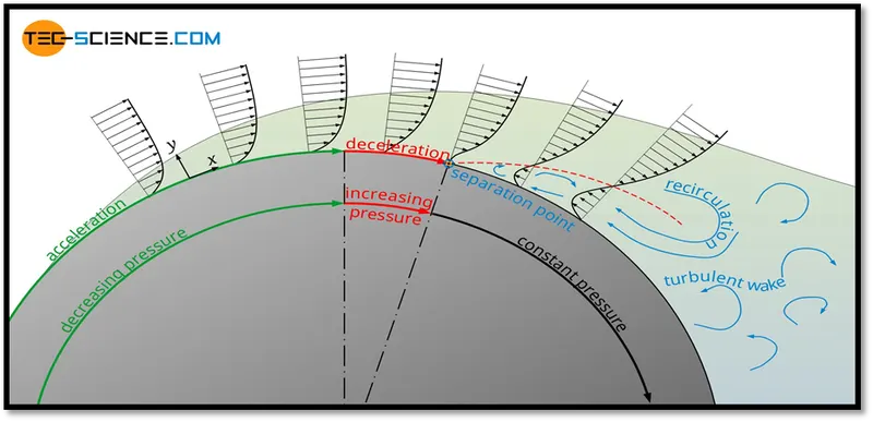
Fig: Velocity direction over a curved surface (du/dy)

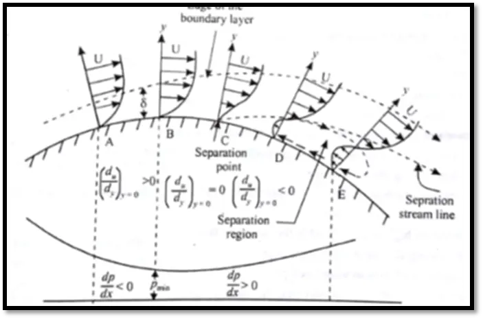
Fig: Velocity profile over a curved surface

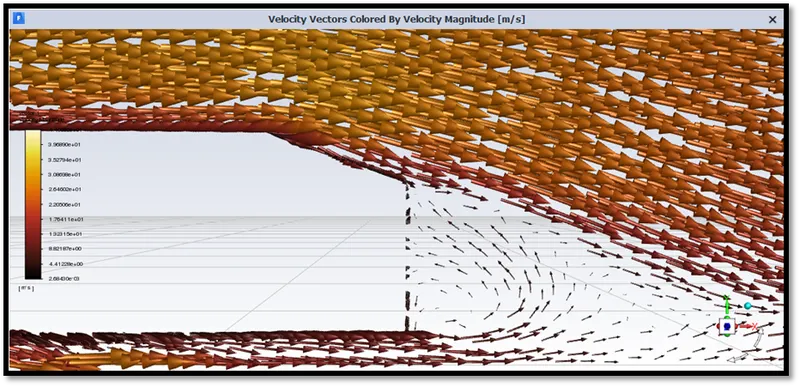
Fig: Velocity vector contour – highly refined mesh (laminar viscous model)

It is the point of separation which causes the change of velocity directions near wall. The wake region has negative pressure gradients. Usually a fluid travels from a point of high pressure to low pressure, which is naturally a phenomenon to determine the flow direction. But in this case, the pressure is low at the wake region, a disturbed flow where the fluid does not detach/disengage from it’s position away from the recirculating zone. This creates pressure drag (blunt body) which must be minimized for better aerodynamics. It simply goes to prove that the fluid will not be in contact with the whole portion of the object and a negative pressure gradient is formed in the wake region.

Thus, a low pressure and velocity region is created as the object is blocking the flow downstream of the point of separation where the velocity is lower than the external flow. A flow reversal takes place considering the effects of the external flow onto the boundary layer and the geometry being a curved surface.

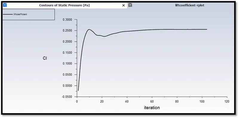
Fig: Coefficient of lift (C_L plot) of k-e model

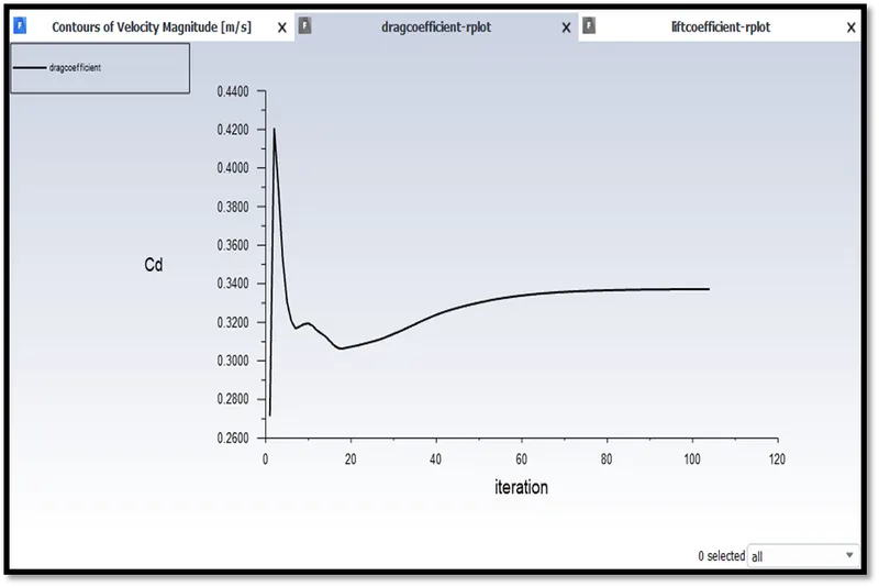
Fig: Coefficient of drag (C_d plot) of k-e model

The drag and lift report values are given below.

Serial Number	Turbulence Model	Lift coefficient value	Drag coefficient value
i)	k-e	0.25520564	0.33716732
ii)	k-w	0.2328394	0.33896408

The k-e turbulence model values vary depending on the mesh element centers and their placements near the wall. However, both turbulence models have given results in the proximity of only 0.531% error by specifying an optimum y+ value in both cases.

Case B – Grid Independency Test

Below are the details for the sub cases i), ii) and iii) corresponding to different element sizes and tending to mesh refinement.

Serial Number	Mesh Element Size (mm)	Lift coefficient value	Drag coefficient value
i) Base-Line Mesh	100	-1.0204032e+42	-3.433681e+39
ii) Refined Mesh	50	0.17061978	0.31219616
iii) More Refined	35	0.22102529	0.31540955

A difference percentage of only 1.024% is found between sub-cases ii) and iii). For the sub-case i), the base line mesh is very coarse as generated by default. This makes the mesh element centers spaced in an unorganized manner which deviates away to capture results effectively. This being the reason, the values recorded are inaccurate and tends to accuracy with better mesh quality and usage of inflation layers near walls.

The drag coefficient plot for the refined model using a laminar viscous model is given below

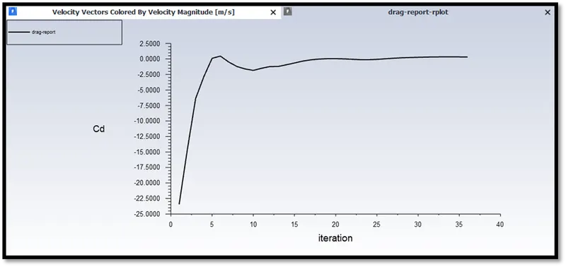
Fig: Drag coefficient plot for refined mesh – laminar viscous turbulence model

CONCLUSION

For Case ‘A’, a difference percentage of only 0.531% is found for drag coefficient values.

A difference percentage of only 1.024% is found between sub-cases ii) and iii) under Case ‘B’. The criterion that differentiates the result values are the mesh size, inflation layers, y+ values, turbulence models and the overall refinement of the enclosures considering the ahmed body.

References

[1] https://volupe.se/en/wall-y-calculator-when-meshing-a-geometry-for-cfd-analysis-this-handy-volupe-calculator-computes-the-height-of-the-first-mesh-cell-off-the-wall-required-to-achieve-a-desired-y-using-flat-plate-boun/ - GOOGLE

[2] Internet sources and information

[3] https://www.ques10.com/p/35971/write-short-note-on-boundary-layer-separation-an-1/

[4] https://en.wikipedia.org/wiki/Fluid_dynamics