Week 2 - Flow over a Cylinder.

Introduction to GUI based CFD using ANSYS Fluent

Flow Over A Cylinder- Report

B A Mayur

INTRODUCTION

For a moving object in fluid, there are normally four forces acting on it i.e., lift, drag, thrust and weight. Here the problem is focused on a stationery cylinder and fluid passing around it for a Reynolds number in the laminar regime. By varying the velocity to increase the Reynolds number, the flow becomes less dense and fewer friction effects cause the flow to create a pattern behind the cylinder in the wake region. This pattern is called the vortex shedding which is seen at a particular Reynolds number and flow velocity as the fluid passes around the cylinder in this 2-D simulation steady flow problem.

For PART I, Case B, an error of 1.077% is found as compared to reference numbered [3], where the drag coefficient is recorded as 1.3353 for a Reynolds number set as 100 of a certain geometry and model simulation.

AIM

• To obtain the flow behavior (vortex shedding) using monitor points 8 meters away from the center of the cylinder within the rectangular computational domain.
• To obtain comparative results of the customized fluid flow pattern by varying the velocity between steady state and transient flow approaches using a laminar flow model.

THEORY OF THE PROBLEM

In this report, the problem statement relates to the flow around a cylinder. By creating a runtime animation of the same, the effects or flow around a cylinder can be visualized by using a laminar viscous flow turbulence model. The cylinder of diameter 2 meters is placed in a rectangular computational domain and one surface of the rectangular computational domain is set as inlet. This flow can be refined to create the vortex shedding, hence it can also be called as “customized fluid”. The physics required to obtain the effect is studied considering numerical diffusion for different mesh domains followed by Von Karman effects, Strouhal number at a certain Reynolds number for steady flow and transient flow approaches. The study is mainly to understand the changes of flow over a cylinder for different input functions to witness the transitioning of flow pattern in the wake region, thus also to simulate the vortex shedding effects.

In a fluid flow dynamics problem, the value of oscillations in an unsteady flow can be used to find the Strouhal number which is a dimensionless value. The numerical diffusion is also countered in this flow problem for both approaches. Usually the vortex shedding is captured if the Reynolds number is above 40 for the customized fluid. This unsteady flow separation around blunt bodies causes a repeated pattern of swirling vortices called the Von Karman vortex effect or the Von Karman vortex street.

GOVERNING EQUATIONS AND OTHER SUPPORTING EQUATIONS

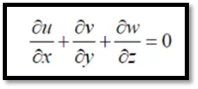
The conservation of continuity, momentum and energy equations is used to calculate the problem and validate the analysis.

Conservation of mass equation:

Conservation of momentum equation:

Reynolds Number (Re):

Re =

Where ‘ρ’ is the density in kg/m³, ‘v’ is the velocity in m/s, ‘D’ is the diameter of the cylinder in meter and ‘μ’ is the dynamic viscosity of the fluid in N/m².

Strouhal Number (St):

Where ‘fst’ refers to the frequency of oscillations, ‘D’ is the diameter of the cylinder and ‘U’ is the velocity of the fluid flow or the inlet velocity as mentioned.

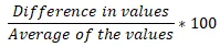
The formula for difference percentage is:

SOLVING AND MODELING APPROACH

The geometry for the computational domain is given in the figure below. The diameter of the cylinder is 2 meters and the corresponding dimensions are given for the computational domain and monitor point.

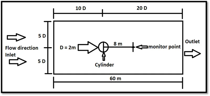
Fig: Dimensions for the simulation model

The dimensions are mentioned and a figure/surface is drawn using SpaceClaim in ANSYS Workbench. They are varied with respect to the center of the cylinder. Each side above and below the cylinder is an inlet surface of 10m, i.e., a total of 20m (left side of rectangular computational domain). The length of the rectangular domain (20m + 40m) is 60m. A laminar viscous model is chosen to solve the flow problem as the Reynolds number is very low, usually in the range 40 to 100 and the transitioning of the vortex shedding is depicted/simulated around these Reynolds number values. A monitor point is created 8m away towards the right from the center of the cylinder along the flow direction.

Firstly a sketch is drawn as shown.

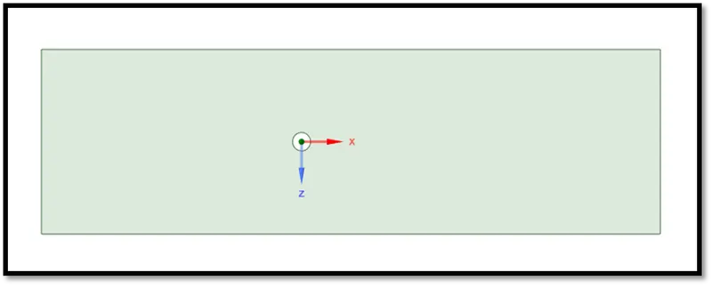
The cylinder is then drawn at the desired dimensions. The domain is converted to surface and that of the cylinder is deleted. This way we get the surface for simulation, both the cylinder and the fluid computational domain to capture the fluid effects. The figure is drawn in the x-y plane and “named selection” feature is used to help setting up the boundary conditions. The upper and lower lengths of the rectangle are set as symmetry walls and the other two surfaces are mentioned as inlet and outlet walls. The cylinder edge is also considered as a stationary wall with no-slip condition for the simulation.

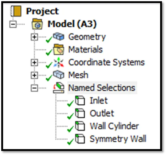
Finally, the desired model is obtained on which the simulation can be performed.

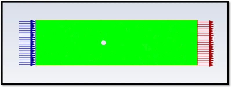
Fig: Flow Over Cylinder- Computational Domain as per the Geometry

The mesh size of the model is set to 0.25m element size. The image shown below is of a triangle dominant mesh. We must make sure that the geometry on top of which we want to simulate the flow are captured perfectly. This calls for the need of a perfect body fitted mesh. The mesh has 23862 nodes, 46760 cells and 70622 faces.

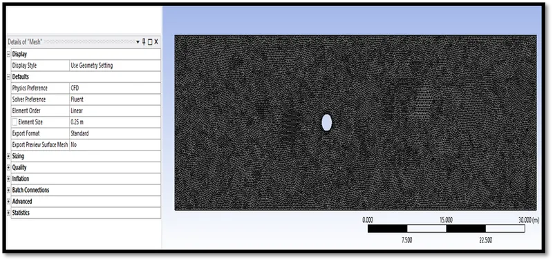
The sizing method is set to “control” the mesh and around the cylinder the number of divisions is set to 36. This means that for every 10⁰, there is a mesh point or node around the edge of the cylinder making them close to the corresponding mesh point. The inflation layer is set to make the mesh fit to the body perfectly with a growth rate of 1.2. This means that for every 120%, the mesh element varies in distance away from the cylinder edge.

In this report, ANSYS FLUENT 2020 R1 is used to capture the results. The solver type is pressure based to solve the steady flow problem. CFD Post is used to anticipate post processing data.

TURBULENCE MODELS

The model specifies options for control of the flow. Here the laminar flow option is selected which specifies that the flow is not turbulent in nature and the flow has a low Reynolds number around 100 by varying the velocity. A pressure based solver is used to proceed with a steady state approach.

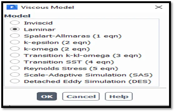
By varying the velocity, the change in the Reynolds number can be optimized. A user defined type fluid or a “customized fluid” is set towards the optimization of obtaining the vortex shedding. The density is 1kg/m³ and thus the chosen turbulence model (laminar viscous model) will be sufficient for the simulation to obtain the results within an expected margin of error for the streamlined flow.

PRE-PROCESSING AND SOLVER SETTINGS

The fluid domain is defined as air and the boundary of the solid-fluid interference is defined as wall. The energy equation is usually turned on to facilitate setting the temperature parameters of the system but here in this case, it is not required as the flow does not need setting up of thermal properties. The velocity at inlet is set to 1m/s. The gauge pressure is equal to 0 as this is the atmospheric pressure (1atm) and the gauge reads zero unless triggered. The boundary conditions for the inlets are velocity type inlets and a pressure based outlet with no specific values set by the user. The backflow pressure specification at outlet is set to total pressure and is solved by the solver after initialization.

Below are descriptive images to show the boundary conditions and solver settings to proceed with simulation using a steady state solver for Reynolds number = 100.

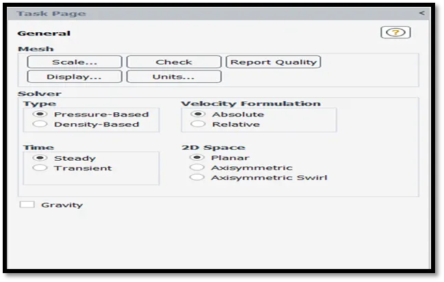
Pressure based solver and a steady state approach is chosen for the simulation. For the unsteady case, the transient approach is chosen.

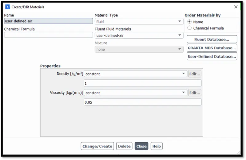
The density of the user defined customized fluid is set to 1kg/m³ with a viscosity of 0.05kg/ms.

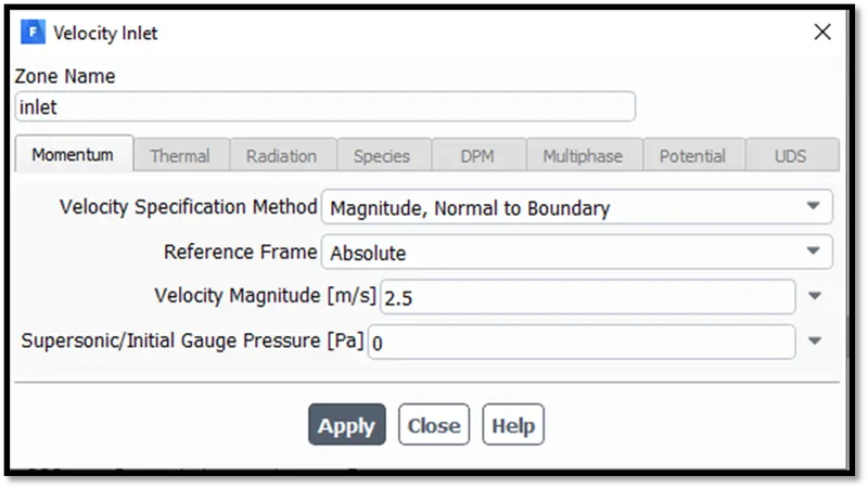
The velocity of the fluid at inlet is set to 2.5m/s.

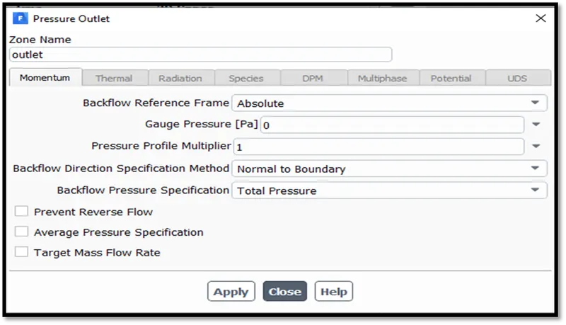
The gauge pressure is mentioned as 0 i.e., 1 atm pressure.

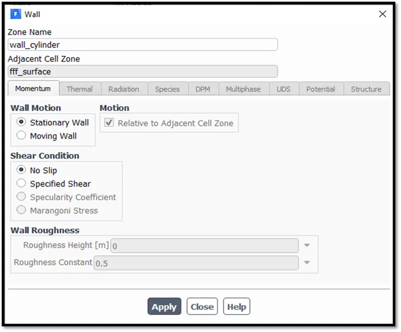
A no slip condition is specified for the flow around the cylinder edges. This helps to consider the friction effects and creating a velocity profile near the wall. At the wall, the velocity is zero. Due to adhesion or intermolecular forces between solid-fluid and fluid-fluid molecular interactions, the molecular attractive forces of the viscous sub-layer have a tendency to resist the movement or rate of change of time of the buffer layer above the wall. This in turn have a relatively lower force being exerted by the layers as progressed away from the wall, thus creating a velocity profile being caused by the viscosity.

RESULTS

PART I

The solvers are set to obtain a comparative table on steady state and transient approaches for Reynolds number being 100. The table below gives the values of Strouhal numbers for both the approaches. The steady state approach is solved for 700 iterations and the transient time state for 500 time steps having 10 iterations per time step. The time step size is specified as 0.1seconds, a total of 5000 iterations.

Case A – Steady state approach

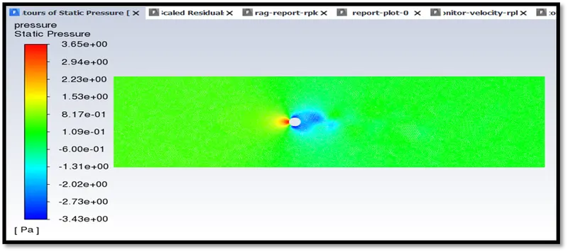
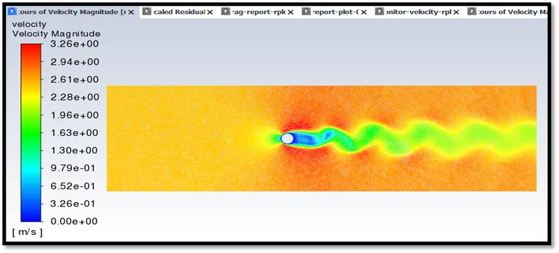
The flow is simulated for the steady state approach. Below are the contours for Re=100.

Pressure contour

Velocity contour

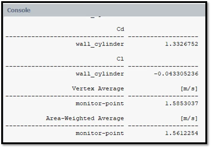
Drag and lift report values are found to be 1.3326 and -0.0433 at the cylinder wall.

The velocity for the monitor point is found to be 1.58m/s.

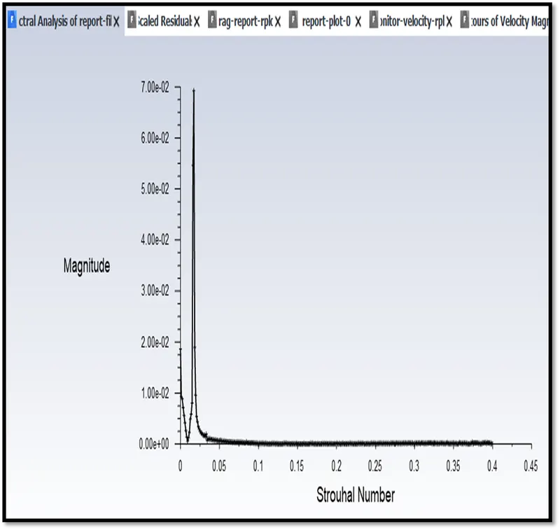
The Strouhal number plot is given below.

The report residuals for the steady state approach are given below.

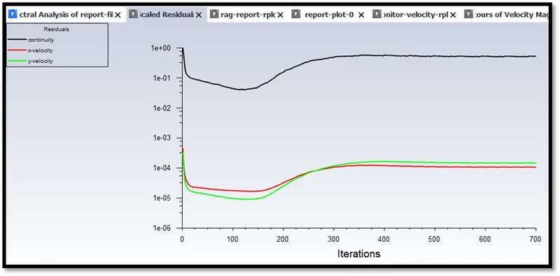
The flow has been converged.

Case B – Unsteady/Transient State Approach

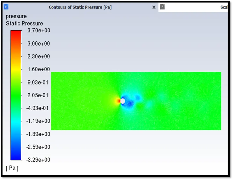
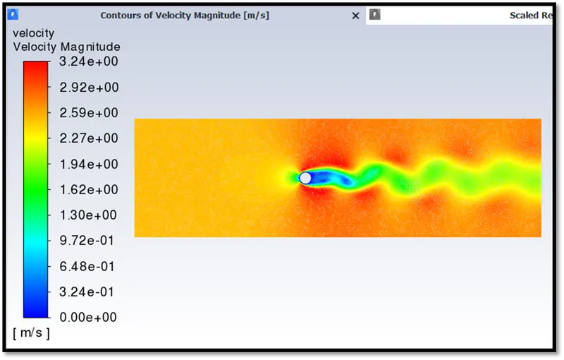
The flow is simulated for the transient approach. Below are the contours for Re=100.

Pressure contour

Velocity contour

Drag and lift report values are found to be 1.3209 and -0.03203 at the cylinder wall respectively.

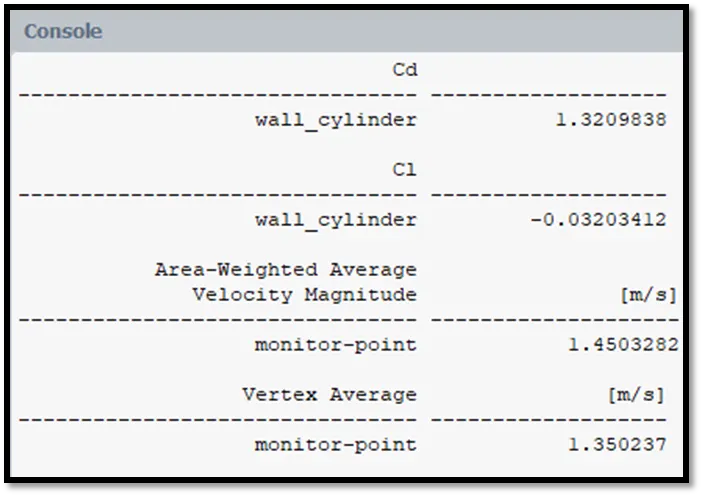
The velocity for the monitor point is found to be 1.35m/s.

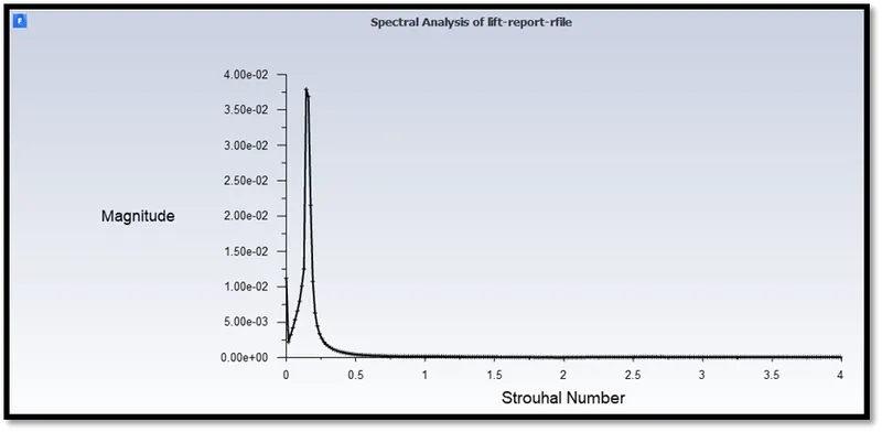
The Strouhal number plot is given below.

The report residuals plot for the unsteady state approach is given below.

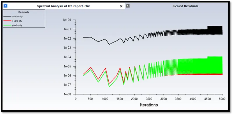
The flow has been converged as the plot show a repetitive pattern of residuals.

The table below shows the values for both simulations obtained.

Function	Steady State Approach (Magnitude)	Transient State Approach (Magnitude)
Strouhal Number	6.92E-02	3.79E-02
Area Weighted Average at monitor point; outlet - Velocity (m/s)	1.5612254; 2.5025606	1.4503282; 2.5034133

PART II

The results in this section contain values for drag and lift coefficients for different Reynolds numbers as mentioned in the table.

Case No.	Reynolds Numbers	Lift Coefficient	Drag Coefficient	Monitor point velocity (m/s)
1	10	-0.0015748318	3.3224911	0.10618738
2	100	-0.043305236	1.3326752	1.5853037
3	1000	-0.38474713	0.8242226	19.810475
4	10000	-0.66726803	0.92173519	176.68041
5	100000	-0.95535226	0.76752721	1870.8507

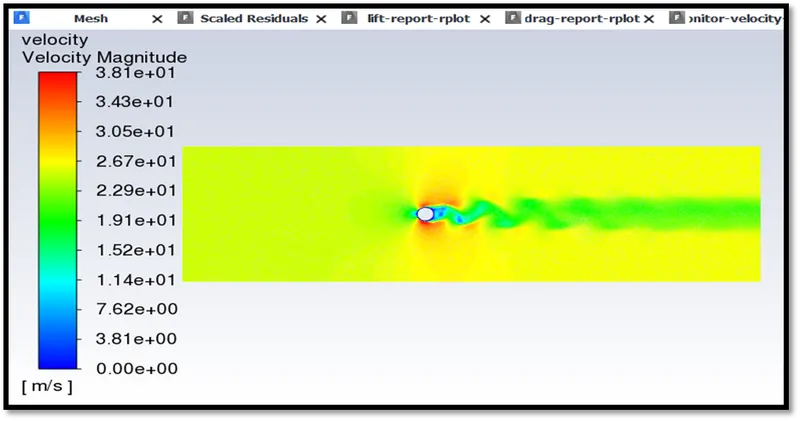
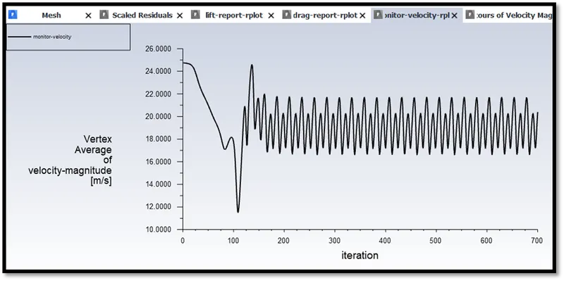
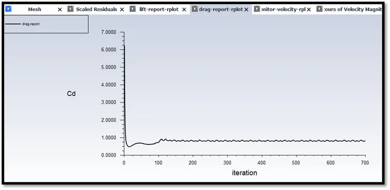
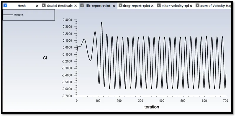
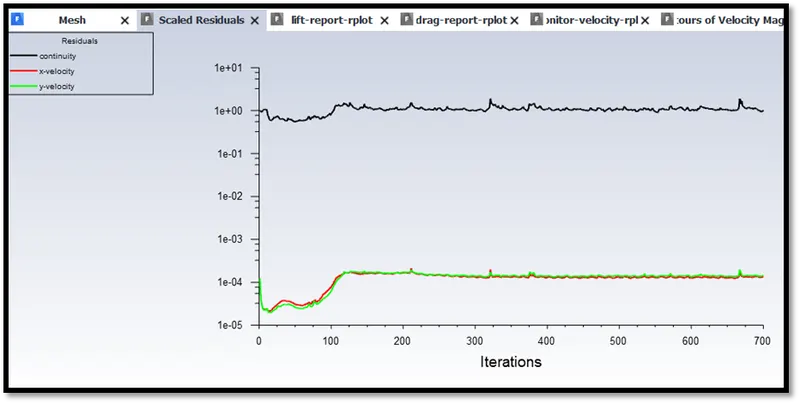
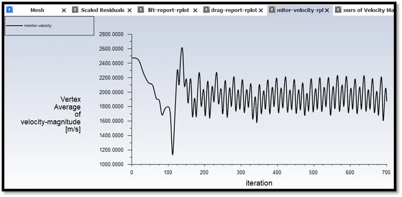
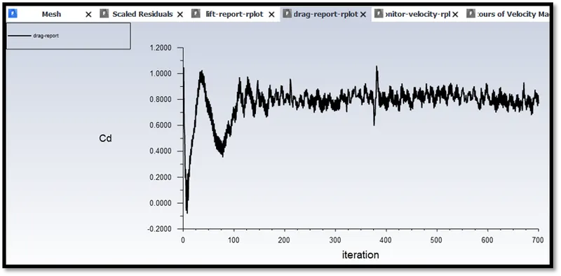
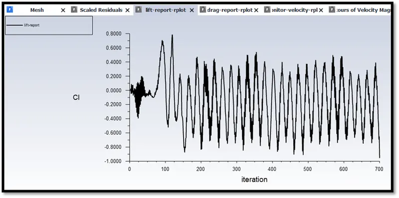
The plots for Re=1000 are shown below. The residuals seem to converge around 140^th iteration for a total of 700 iterations. We can say this as the plots show a repetitive pattern for the residual curves. The vortex shedding is seen in the velocity magnitude plot showing a maximum of 38.1m/s in it’s legend. However, a value of 19.81m/s is noted at the monitor point for this simulation and values around 24.9m/s are noted at outlet. A difference average of 174.88% is noted between case number 1 and 2 for velocity values at monitor point.

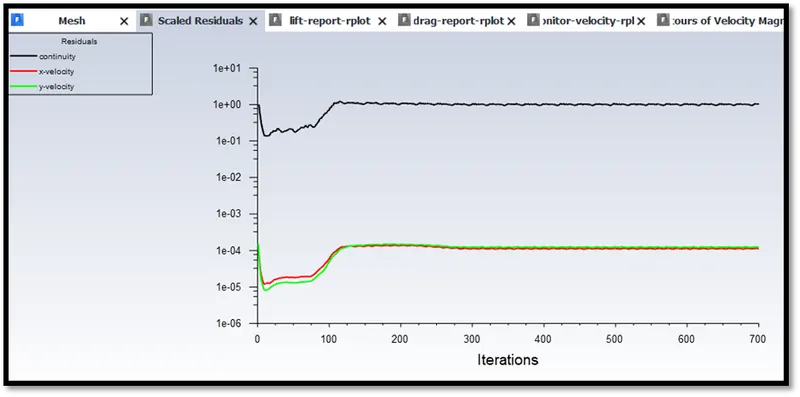
The plots for Re=100000 are given below.

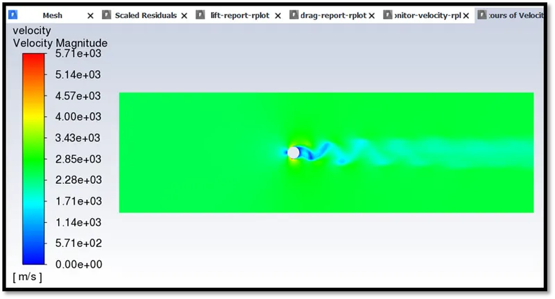
The table below shows the recorded drag coefficients for different Reynolds numbers at the monitor point. The calculations are solved for 700 iterations, sufficient to succumb to the convergence criteria.

Reynolds Number	Drag Coefficients	Difference Percentage (%)
10	3.3224911
100	1.3326752	85.4884
1000	0.8242226	47.1466
10000	0.92173519	11.17
100000	0.76752721	18.2574

CONCLUSION

The velocity at monitor point increases due to the increase in Reynolds number for viscosity remaining the same i.e., 0.05kg/(m-s). The vortex shedding pattern occurs alternating in nature due to the low pressure zones that are created in the wake region. The pattern is mainly due to the pressure differences which give rise to the fluctuating forces acting at right angles to the wind direction in the downstream side of the cylinder.

As the flow develops at the bottom of the cylinder to produce the vortex flow pattern in the downstream region, the time here is being utilized for the flow over/above the cylinder to be developed. This is solely due to the pressure difference which causes the alternating pattern of the vortex street thus creating the Von Karman effect.

The laminar viscous model can be used for Reynolds numbers as high as 100000 because we get the desired results for this particular laminar flow problem and we are not interested in the turbulence caused during the simulation. The hybrid initialization option helps us to set pre-defined values before the actual calculation starts. This way FLUENT helps us to solve the pressure and velocity parameters before-hand to initiate the calculation within the environment.

Mainly the Strouhal number is depicted as maximum at 0.0692 at a magnitude of 0.0171 and 0.0379 at a magnitude of 0.144 for the steady and transient state approaches respectively.

In part I, both cases have a repetitive pattern in their respective residual plots. This simply means that between each and every iteration there is a negligible difference value (usually in the range of 1e-3) remaining, which is a very low value. These values seem to be occurring as a loop while solving the governing equations and hence we can say that the solution is converged.

We must note that the lift coefficient values, drag coefficient values and velocity at the monitor point values, all are rather fluctuating corresponding to their own boundary conditions respectively (not constant but close to 0) within a certain range in accordance to the turbulence model. This means that for every iteration, the values lie in the range of two limits. They are not static values but fluctuate with time. These are the values found or recorded based on the number of iterations specified and the value corresponding to that particular n^th iteration for the simulation calculations. Thus when the range for drag coefficients are looked upon, they have a more defined range with an increase in Reynolds numbers. This depends on the mesh parameters as well. The drag coefficients take lesser time to stabilize with an increase in Reynolds numbers.

References

[1] A reference solution of the flow over a circular cylinder at Re = 40 R. Gautier, D. Biau, E. Lamballais ⇑ Institut Pprime, CNRS, Université de Poitiers, ENSMA, Téléport 2, Bd. Marie et Pierre Curie, B.P. 30179, 86962 Futuroscope Chasseneuil Cedex, France

[2] https://dragonfly.tam.cornell.edu/teaching/mae5230-tritton-chap3.pdf

[3] Numerical simulation of laminar flow past a circular cylinder B.N. Rajani , A. Kandasamy, Sekhar Majumdar a, a CTFD Division, National Aerospace Laboratories, Airport Road, Bangalore 560 017, India b Department of Mathematical and Computational Sciences, National Institute of Technology, Karnataka, Surathkal 575 025, India