Week 4 - CHT Analysis on Exhaust port

Introduction to GUI based CFD using ANSYS Fluent

CHT of In-Line 4 Cylinder Exhaust Port - Report

B A Mayur

INTRODUCTION

An exhaust port is useful to vent out the gases post combustion of an internal combustion automobile. Here, the geometry of an in-line 4 cylinder exhaust port is taken which means hot fluid at all four inlets with similar mass flow rates are set and simulation performed to visualize and study the effects of the exhaust port in a conjugate heat transfer approach. The effects of the heat exchanges between the solid and fluid domains are considered by specifying the heat transfer coefficients and setting up a convective wall at the solid-fluid interface to ensure the CHT approach.

Keywords: CHT (Conjugate Heat Transfer), Heat transfer coefficient, Reynolds Number

AIM

• To understand and simulate the conjugate heat transfer process
• To obtain the wall/surface heat transfer coefficient on the internal solid surface & show the velocity & temperature contours in appropriate areas.
• Verification of heat transfer coefficients and factors affecting the HTC predictions obtained from simulations.

THEORY OF THE PROBLEM

In this report, the problem statement relates to the flow within a duct or pipe thus representing the exhaust port. There are four inlet ports and all are vented out to a single common outlet exhaust port. The diameters of all the inlet ports being the same implies that the mass flow rates for these pipes are similar. Therefore the pressure at the start of the exhaust will be relatively higher within the geometry thus simulating higher fluid velocity inside the exhaust bent pipe to accommodate the mass flow rates of four inlet ports. This classic problem is used to depict the study of dissimilar temperatures of the inlet and exhaust ports where the inlet fluid temperature is significantly higher near inlets. Due to the solid-fluid interaction and uneven distribution of number of inlet and outlet ports, the conjugate heat transfer approach is used to study the effects of an internal combustion engine, in-line 4 cylinder automobile exhaust port.

GOVERNING EQUATIONS AND OTHER SUPPORTING EQUATIONS

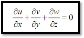
The conservation of mass, momentum and energy equations are used to calculate the problem and validate the analysis.

Conservation of mass equation:

Conservation of momentum equation:

Reynolds Number (Re):

Where ‘ρ’ is the density in kg/m³, ‘v’ is the velocity in m/s, ‘D’ is the diameter of the cylinder in meter and ‘μ’ is the dynamic viscosity of the fluid in N/m².

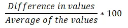
The formula for difference percentage is:

Mass Flow Rate Formula:

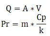
Here, m (mew/mu) = 0.00001813 Pa.s

Nusselt Number Formula:

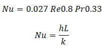
Convective heat transfer coefficient, characteristic length in ‘m’ and thermal conductivity of air = 0.0242W/mk.

Convective Heat Transfer Coefficient – Newton’s Law of Cooling Equation:

Where ‘Q’ is the mass flow rate in kg/m³, ‘A’ is the area of cross section in m² and ‘V’ refers to the velocity of the fluid. The equation represents the mass flow rates at two varying cross-section being same for a given fluid. For a smaller diameter cross-section, the velocity of the fluid will be high to accommodate the mass flow rates of larger diameters prior to this section. In other words, the 1 outlet section has to accommodate the mass flow rates of 4 inlets. Hence the temperature and velocity will be higher at outlet section.

The Dittus-Boelter co-relation works best for smooth circular pipes with minimal temperature differences. The equation helps to understand the local Nusselt number with moderate temperature differences considering the viscosity near wall and that of the bulk fluid.

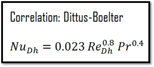
Where, Re refers to the Reynolds number, D_h is the circular pipe diameter and Pr refers to the Prandtl number.

‘μ’ (in Ns/m²) refers to the dynamic viscosity and C_p is the specific heat capacity in kJ/kg-K. ‘k’ is the thermal heat conductivity in W/mK. Using the equation is sufficient to obtain close results for Nusselt Number, thereby obtaining the HTC value.

Problem statement: In this problem, there are four inlets vented out to one outlet section. To accommodate the Q=A*V equation, the mass flow rates vary between these two sections. Thus the conditions and geometry describes the various effects encountered during the simulation considering streamlines, velocity, pressure contours and post-processing visualization.

SOLVING AND MODELING APPROACH

The geometry of the exhaust port is given in the figure below. The dimensions are shown in SolidWorks software after conversion of the geometry file to a step file from SpaceClaim. The figures are a representation of the front view and top view geometric dimensions.

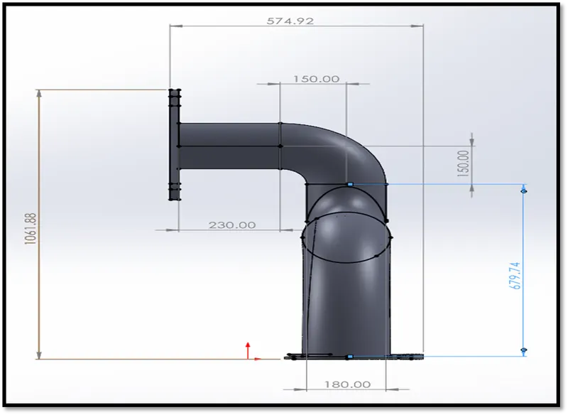
Fig: Dimensions of the simulation model –Front Plane

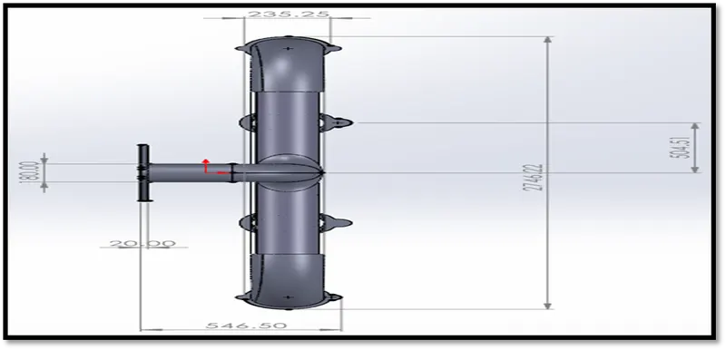
Fig: Dimensions of the simulation model –Top Plane

The dimensions are mentioned in the above figures and a fluid volume extract is taken to understand the flow. We are not interested with the flow over or around the exhaust port, hence there is no need of creating a computational domain or enclosures unless the heat arising from the solid interface of the outer exhaust port must also be considered but that is not the case. Apart from naming the convective wall to set the boundary conditions, the exhaust port mounts are set as adiabatic walls, which mean there is no heat exchange taking place here. Named selections option is chosen to apply boundary conditions for inlets (x4), one outlet and convective wall at the solid-fluid interface. The extra edges in the geometry are removed using the ‘repair’ tool. This tool automatically removes the unwanted edges to help advance in setting up the volume extract. To ensure that the mesh is uniform at this interface, “SharePrep” option in ANSYS Workbench is used to enable a shared topology for conformal mesh intersections between inner region of the solid block and outer region of the fluid volume extract to avoid grid shocks against inaccurate results. The pink coloured circles show where the information is being shared, from inlet to outlet. This means that there is only one interface between solid block and fluid block throughout the geometry. In this way, the heat transfer information can be shared or “exchanged” with accuracy for an efficient CHT approach.

The solid and fluid volumes are then clubbed under a new component renamed as “Final Geometry”. Other empty components are deleted from the feature tree.

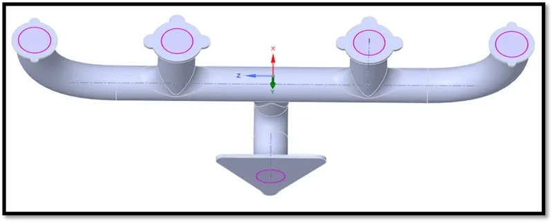
Fig: Information shared between pink inlets and outlets for CHT

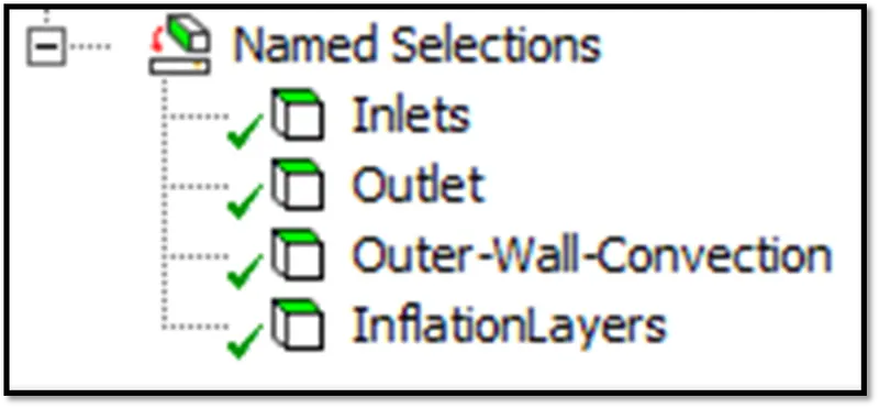
Fig: Named selections

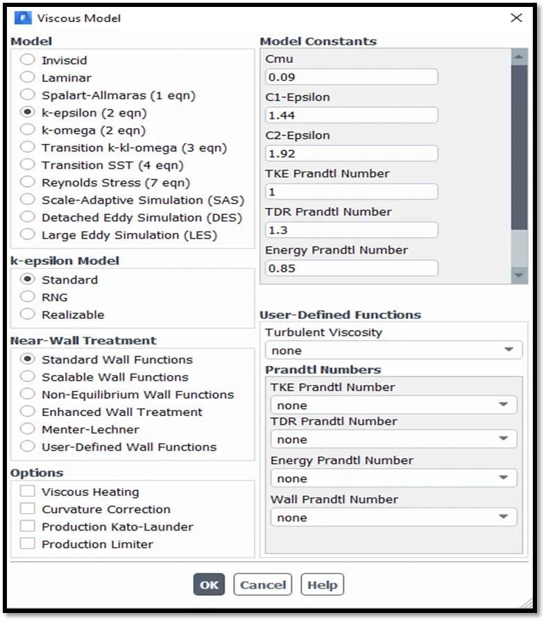
A base mesh is created and then re-defined to a higher degree to capture the flow effects with the application of inflation layers close to the volume extract with a growth rate of 1.2. A k-e turbulence viscous model is used to solve the problem with a steady state approach and a pressure based solver as the Mach number is less than 0.3.

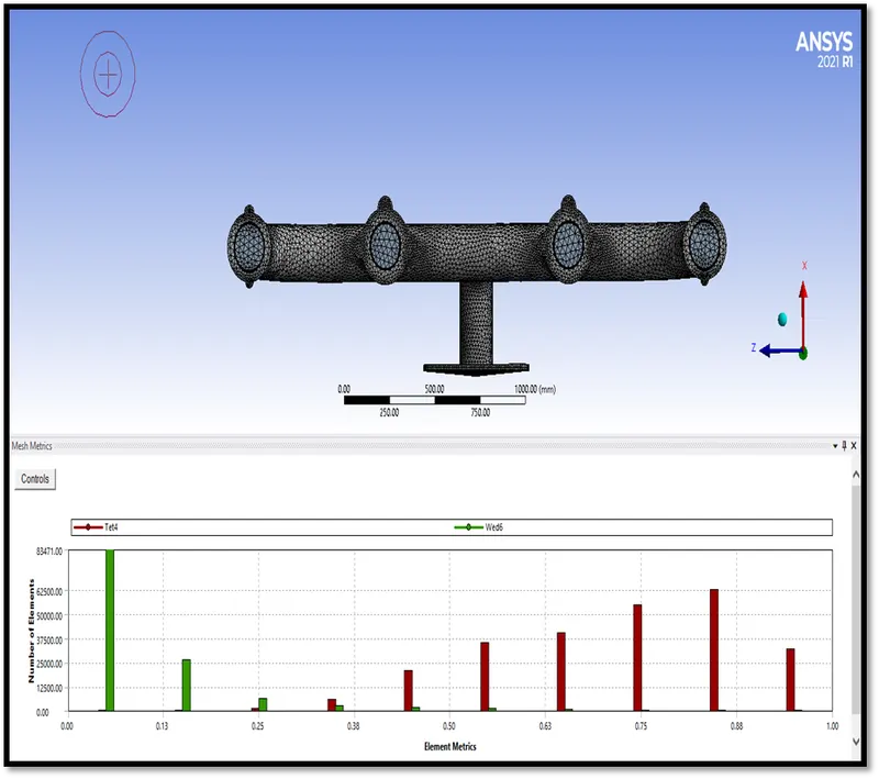
Fig: Exhaust Port Mesh Setup

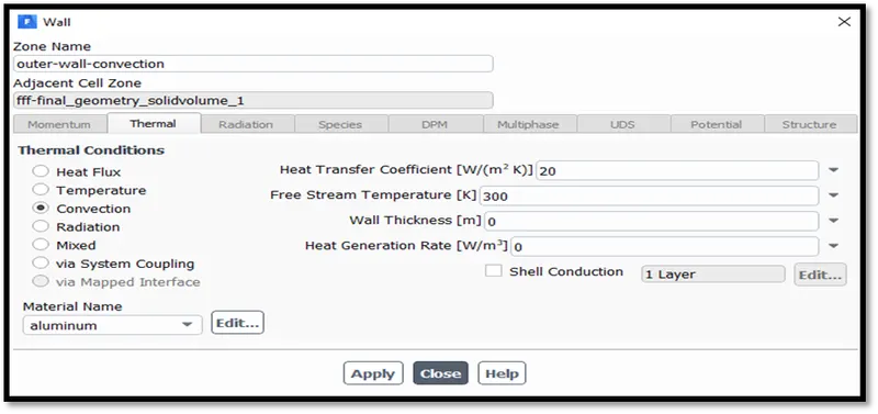
This calls for a perfect body fitted mesh to enable the simulation effects close to the walls with an optimum y+ value. However other settings are set to default for the turbulence model. The units are set to meters on SpaceClaim as the geometry was imported. In the real world, the exhaust port is cooled by air which has a particular heat transfer coefficient. This value is taken as the input which depends on the Reynolds number of the external air flow. Hence the heat transfer coefficient value that has been set will determine the heat transfer rate, also to help produce the post-processing visualizations.

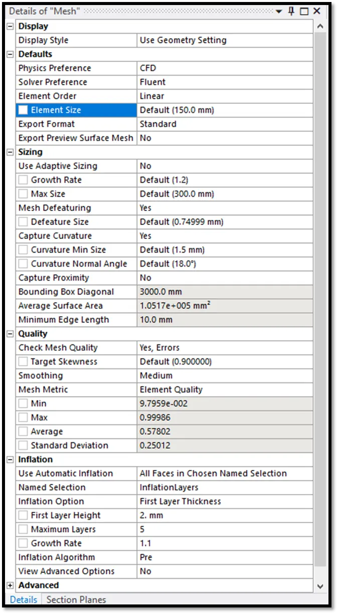
Fig: Mesh Details of k-e model

The mesh details are shown in the above picture and a table follows the mesh details for the different simulations recorded for this report.

Mesh Details Table
	Element Size (mm)	Cells	Faces	Nodes
i) k-e model	150	1396292	3176153	473474
ii) k-w model	150	1391002	3163499	471303

The table above shows the values for number of cells, nodes and faces for the overall mesh element size specified for k-e and k-w models.

TURBULENCE MODELS

The model specifies options for control of the flow. Here the k-e turbulence model works for capturing the results away from the wall, efficiently. The k-w turbulence model captures the flow effects accurately near wall at adverse pressure gradients. Hence a higher y+ value is required for k-e (around 50) and y+ value of 1 or more will be sufficient to capture the results using the k-w turbulence model.

As the velocity is very low, the y+ values for the turbulence models vary between 1-5 and 30-300 for the k-w and k-e models.

PRE-PROCESSING AND SOLVER SETTINGS

Energy equation is turned ON to set up the thermal parameters and solving conservation of energy equations. This enables to solve for the heat transfer between the solid-fluid blocks.

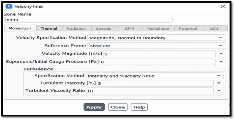
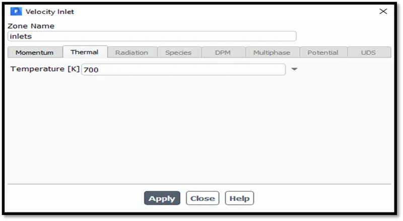
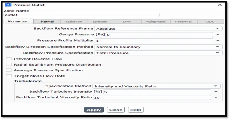
The fluid domain is defined as air and the boundary of the solid-fluid interference is defined as a convective wall. The energy equation is usually turned on to facilitate setting the temperature parameters of the system. The velocity at inlets is set to 5m/s. The gauge pressure is equal to 0 as this is the atmospheric pressure (1atm) and the gauge reads zero unless triggered. The boundary conditions for the inlets are velocity type inlets and pressure based outlets. The backflow pressure specification at outlet is set to total pressure and is solved by the solver after initialization. The temperature of the fluid is set to 700K at inlet.

Below are descriptive images to show the boundary conditions and solver settings to proceed with simulation using a steady state solver for the k-e turbulence model.

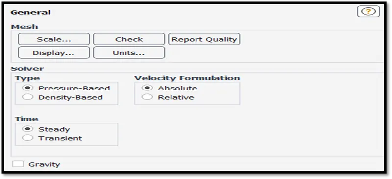
Pressure based solver and a steady state approach is chosen for the simulation.

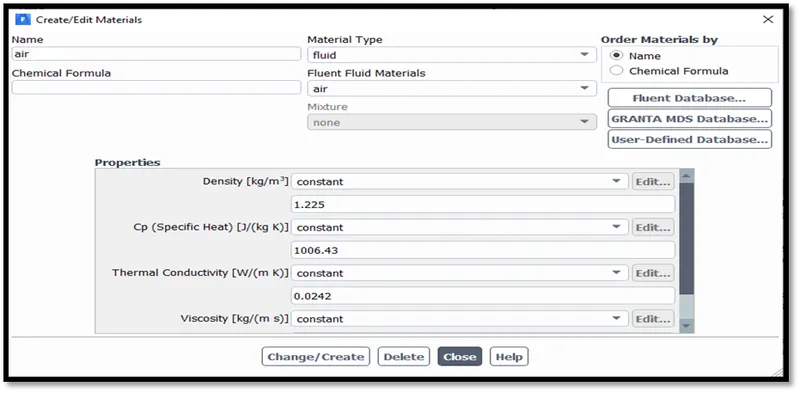
The density of the fluid (air) is set to 1.225kg/m³ with viscosity set as a constant.

The velocity of the fluid at inlet is set to 5m/s.

The temperature is set to 700K for the hot inlet fluid.

The gauge pressure is mentioned as 0 i.e., 1 atm pressure.

The convective heat transfer coefficient is set to 20 W/m² K for the outer convective wall.

All other settings are kept as default.

RESULTS

200 iterations were performed for each model.

CASE ‘A’ – k-e and k-w Turbulence Models

1. The k-e turbulence model

In this section, the k-e turbulence model solves two transport equations (PDEs) to encounter the effects more accurately at regions away from the wall. Hence to capture the flow effects near walls, a y+ value of 50 is required.

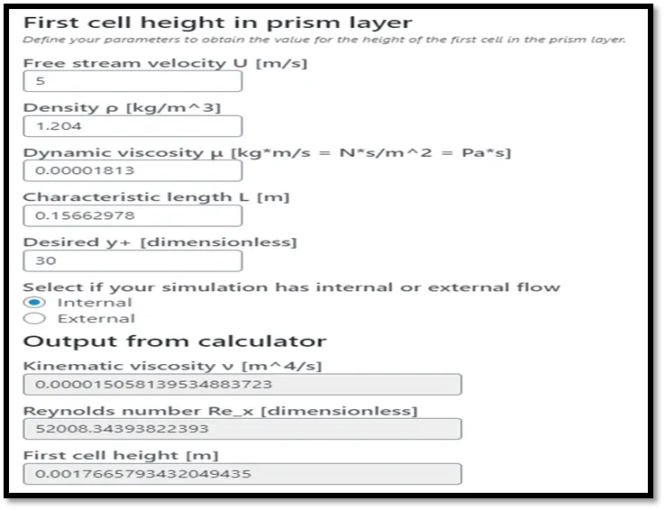
Fig: y+ value for k-e turbulence model

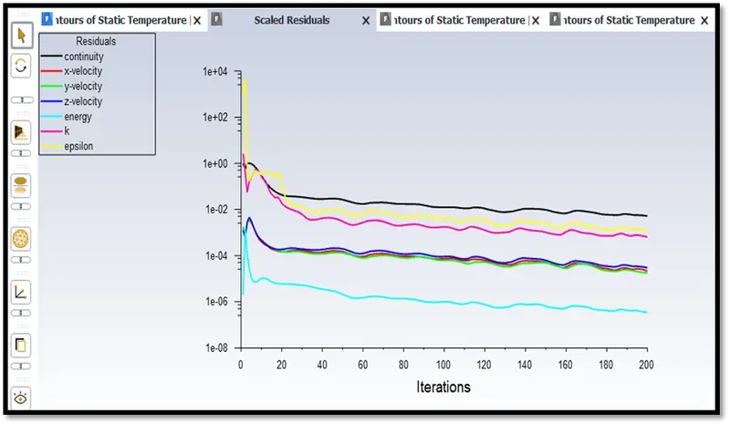
Fig: Scaled residuals plot – k-e turbulence model

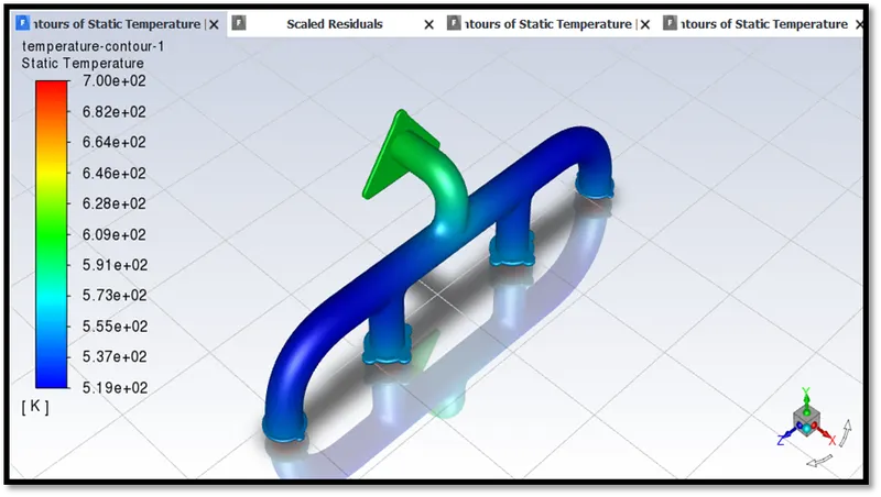
Fig: Temperature contour of k-e turbulence model

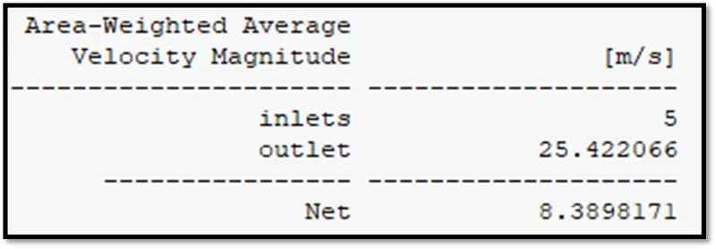
Fig: Velocity values – k-e turbulence model

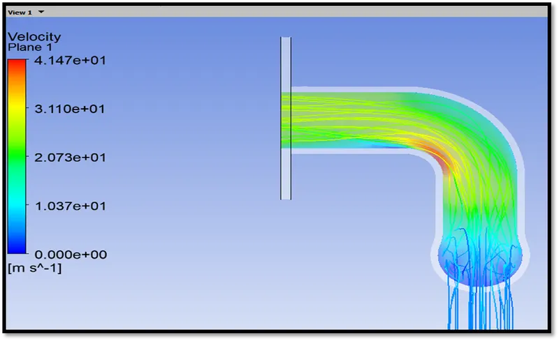
Fig: Velocity contour at outlet pipe – k-e turbulence model

1. The k-w turbulence model

The k-w turbulence model is best used to capture the near wall effects at adverse pressure gradients. Thus a y+ value of only 1 is sufficient to capture the effects near the walls to define the inflation layers.

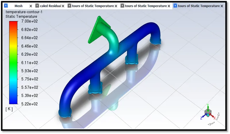
Fig: Temperature contour of k-w turbulence model

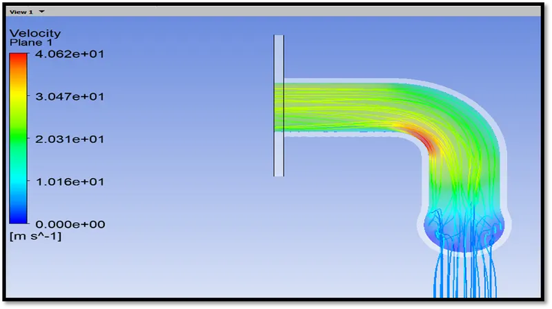
Fig: Velocity contour at outlet pipe – k-w turbulence model

Sl.No.	Turbulence Model	Temperature values (K)	Percentage difference (%)
1.	k-e turbulence model	675.78881	------
2.	k-w turbulence model	675.29611	0.072933

The heat transfer coefficient is the proportionality constant between the heat flux and the thermodynamic driving force (temperature difference) that drives the heat flow and is used to calculate the heat transfer.

The verification of heat transfer coefficient

Dittus-Boelter equation – Nusselt Number	HTC value in W/m2K	Difference Percentage (%)
116.571	16.994	16.25

CONCLUSION

The simulation was performed for both the k-e and k-w turbulence model and temperature values were found with a difference of only 0.073%. The heat transfer coefficient was calculated theoretically and found to be W/m²K. The value deviates by only % than the original HTC value which is 20W/m²K.

The HTC value has an error of 16.25% which deviates from 20 W/m²K. The Dittus-Boelter formula works efficiently for flow in smooth circular pipes. In this case, the exhaust flow pipe is of a different geometry as there is a bend in the pipe. This causes inaccuracy in obtaining the HTC values and the error calculated is 16.25%.

References

[1] y+ calculator online link - https://volupe.se/en/wall-y-calculator-when-meshing-a-geometry-for-cfd-analysis-this-handy-volupe-calculator-computes-the-height-of-the-first-mesh-cell-off-the-wall-required-to-achieve-a-desired-y-using-flat-plate-boun/ - GOOGLE

[2] Internet sources and information

[3] Internet information link - https://www.nuclear-power.com/nuclear-engineering/heat-transfer/convection-convective-heat-transfer/dittus-boelter-equation/

[4] Wikipedia website link - https://en.wikipedia.org/wiki/Fluid_dynamics