Week 1- Mixing Tee

Introduction to GUI based CFD using ANSYS Fluent

Mixing Tee Report

B A Mayur

Introduction

The mixing of cold and hot fluids stimulates a variety of results. This stirs up the engineering of maintaining the approximate cold fluid inlet temperatures that mixes with the hot fluid to get a desired outlet fluid temperature. The model that helps perform the objective is called a mixing tee of a desired geometry.

In this report, cases are depicted using a short and long mixing tee geometry. The standard deviation and area weighted average at the outlet is presented for the outlet section and the contours are shown to understand what exactly happens within the volume extract, inside the solid material at mid-section of the steady flow problem.

AIM

• To obtain an approximate average of the two hot and cold inlet fluid temperatures at outlet section and validating using k-e and k-w models followed by grid independence test for two mixing tee geometries.
• This is achieved using the standard deviation chart values to validate the effectiveness at the outlet section. The area weighted average gives an estimate of the temperatures of the fluid at outlet thereby checking for mixing effectiveness.

THEORY OF THE PROBLEM

In this report, the problem statement relates to the mixing of two fluids, to finally get a fluid relative to the temperatures of the initial mixture.

The fluid interaction happens at maximum efficiency when they intersect perpendicularly, thereby enhancing turbulence and disturbing the homogeneity, the fluid inlet flows being at different velocities.

GOVERNING EQUATIONS AND OTHER SUPPORTING EQUATIONS

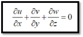
The conservation of continuity, momentum and energy equations are used to calculate the problem and validate the analysis.

Conservation of mass equation:

Conservation of momentum equation:

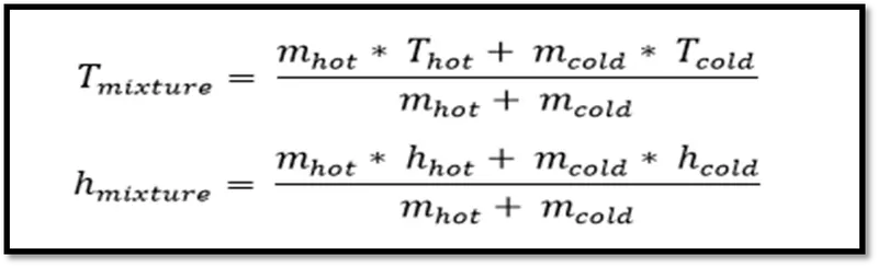
The formulae for calculation of the T_mixture is used to get the analytical results.

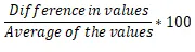
The formula for difference percentage is:

SOLVING AND MODELING APPROACH

The geometries of both the mixing tee i.e., short and long vary in dimensions of the main axial cold inlet flow pipe. The diameter and length of the vertical pipe which houses the inlet for the hot fluid is designed to be of same length for both cases.

Basically the pipes are joined close to the inlet section and a decent length is provided to anticipate the mixing efficiency. This is touched on two cases and analysis performed for different velocities to check the standard deviation and efficiency of mixing affecting the fluid at outlet section.

The diameters of the cases are shown below.

MIXING TEE CASE	HORIZONTAL DIAMETER (HOT FLUID INLET-OUTLET) in ‘m’	VERTICAL DIAMETER (COLD FLUID INLET) in ‘m’	LENGTH OF THE HORIZONTAL PIPE in ‘m’
A - SHORT	0.03	0.02	0.2
B - LONG	0.03	0.02	0.27

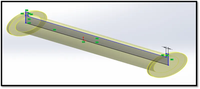
Firstly a sketch is drawn as shown.

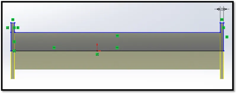
It is then followed by a revolve feature to get the desired shape of the geometry. This gives us the mixing tee model. The same procedure is followed to get the model for case B according to the given dimensions as shown in the previous table.

Finally, the desired model is obtained on which the simulation can be performed.

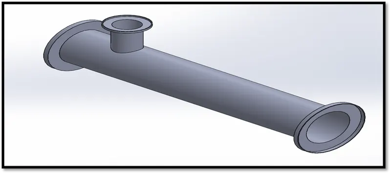
Fig: Mixing tee Short

The mesh size of the model is set to 5e-5 mesh size. The image is shown below.

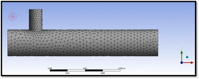
In this report, ANSYS FLUENT 2020 R1 is used to capture the results. The solver type is pressure based to solve the steady flow problem. CFD Post is used to anticipate post processing data.

TURBULENCE MODELS

SST stands for shear stress transport. The k-e and k-w vary in solving equations accurately and provide better results at wall (near wall treatment) at adverse pressure gradients. Hence k-w model is best used for near wall treatment solutions. The k-e model solves the 5e-3 mesh for the short mixing tee accurately and close to the analytical results with an error of only 1.736%. However in this report the simulation is done using the k-e turbulence model because the area of interest for the given output is off the walls. We are looking for accuracy in the free surface flow region, pressure plots or contours not being our primary concern for these cases than the temperature and velocity information. Also, the k-e turbulence model provides a coser value to analytical results for both the 3e-3 and 5e-3 mesh which can be considered as it takes lesser time to converge. The details are mentioned after the table which follows the image below.

K-e and k-w models are tested and compared to check the variation of outlet temperature results. A mesh size of 3e-3 is chosen and run for both models of the short mixing tee model as well as for the 5e-3 mesh.

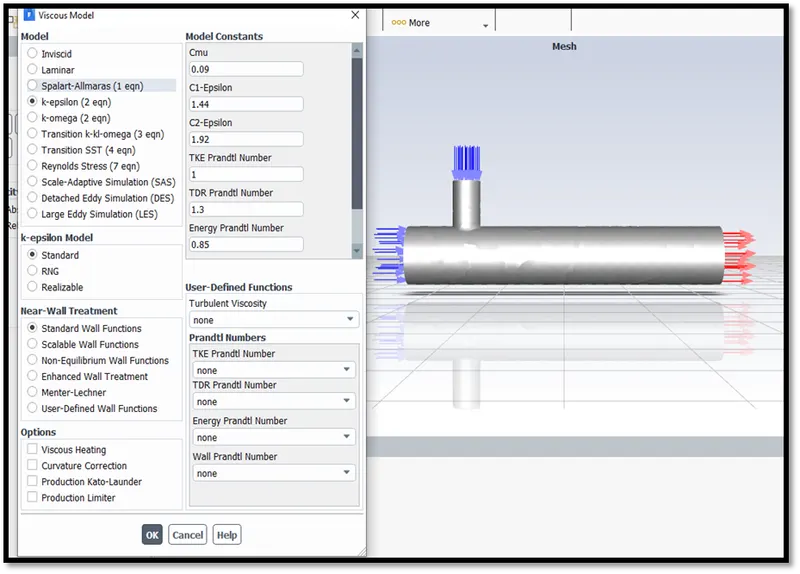
The results are as shown below and checked for 350 iterations in comparison to the analytical results for the short mixing tee.

Mass flow rate of COLD FLUID (A*V) = 6 m/s* 0.00027348075 m²

Mass flow rate of HOT FLUID (A*V) = 3 m/s * 0.00093505914 m²

T_hot = 36⁰C

T_cold = 19⁰C

Sl. No.	k-e model	k-w model	Analytical results Tmixture
1. (3e-3 mesh size)	30.258486 0C	30.32277 0C	29.72590013 0C
2. (5e-3 mesh size)	30.241988 0C	30.283158	29.72590013 0C

The error is 1.79% for the k-e model from analytical results. The results are close to analytical results for the 5e-5 mesh with an error of 1.7361%.

A standard deviation for k-e model was obtained as 2.0773765 ⁰C and 1.9427973 ⁰C for the k-w viscous model. This is for the 3e-3 mesh size.

For the 5e-3 mesh size the results obtained were 1.7840401 and 1.5766281 for k-e and k-w turbulence viscous models respectively.

The solution for the standard realizable k-e model was converged at 163^rd iteration. The solution for the standard realizable k-w model was converged at 188^th iteration.

It can be noted that the k-e turbulence model for the 5e-3 mesh size gave closest results to the analytical results.

The mixing tee design model has been meshed to get an optimum range of results for validation. A grid independence test was performed and graphs plotted to show the variation in results for mesh models as shown in the table below. For case A, a sizing of 5e-3 and case B sizing of 1e-3 was given to the mesh model.

Mesh Model – Mixing Tee Short	Cells	Nodes	Faces
8e-3 mesh size	12583	2797	26451
5e-3 mesh size	14247	3142	29907
3e-3 mesh size	39817	8350	82882
1e-3 mesh size	573264	110098	1174734

A volume extract is taken as we are interested in the property changes that occur to the fluid and that the study is not of conjugate heat transfer where the solid domain must be considered for heat transfer between the two domains.

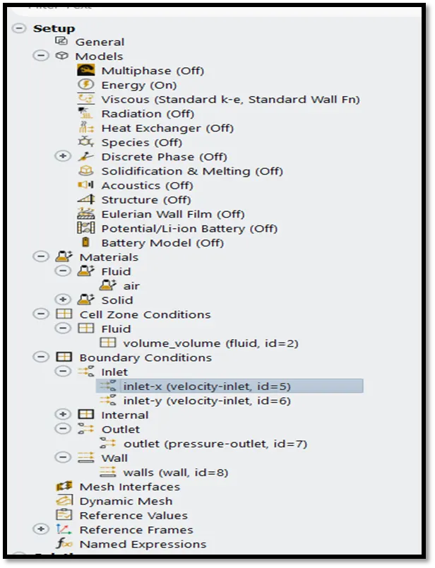
The inlet sections and outlet section are named along with the wall to set up the boundary conditions. These details are described in the section below.

PRE-PROCESSING AND SOLVER SETTINGS

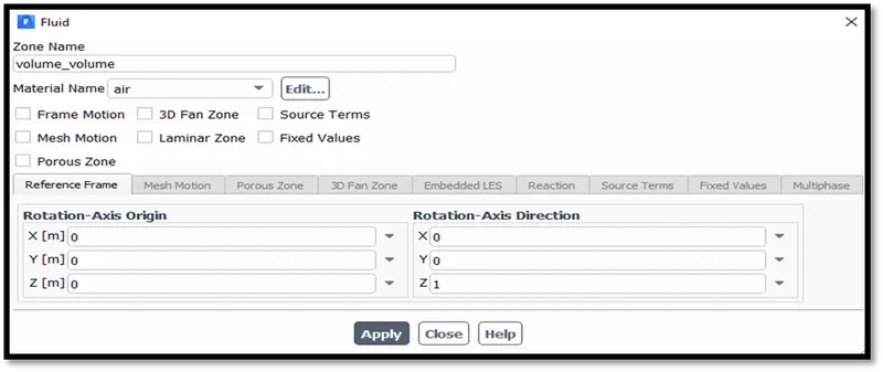
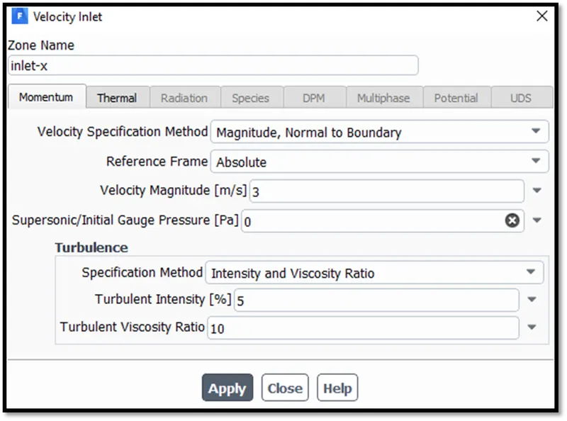
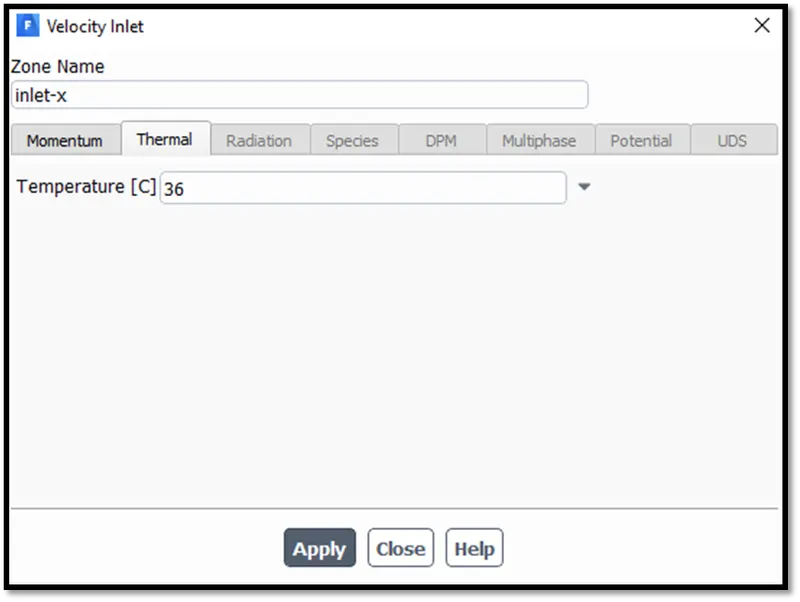
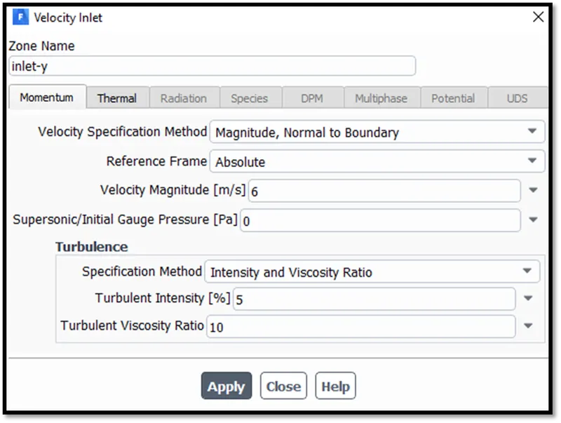
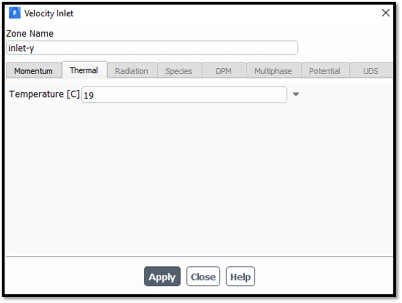
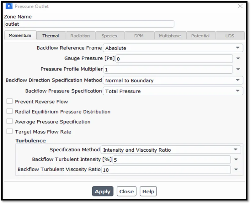
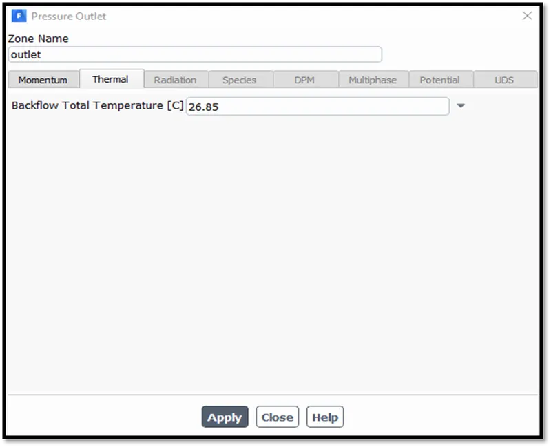
The fluid domain is defined as air and the boundary of the solid-fluid interference is defined as wall. Firstly the energy equation is turned on to facilitate setting the temperature parameters of the system. The energy at inlet is set to 3m/s for the horizontal pipe and at 6 m/s for the vertical pipe for case A. The inlet y (vertical) is set to 10m/s for case B. A turbulent intensity of 5% and turbulent viscosity ratio of 10 is used for all the simulation cases. The guage pressure is equal to 0 as this is the atmospheric pressire (1atm) and the guage reads zero unless triggered. The boundary conditions for the inlets are velocity type inlets and a pressure based outlet with no specific values set by the user. The backflow total pressure is solved by the solver after initialisation.

GRID INDEPENDENCE TEST

For all the simulations for the under-given table, the hot fluid inlet velocity has been set to 3m/s at 36⁰C and the cold fluid inlet velocity being 6 m/s, temperature set at 19⁰C using the k-e turbulence model.

For the grid independence test, a coarse mesh size of 8e-3 is taken and simulations performed towards finer mesh size of 1e-3. The results are articulated to be validated.

Mesh Size	Standard Deviation '0C'	Area Weighted Average (Temperature) '0C'
8e-3	1.8064466	30.200366
5e-5	1.7840401	30.241988
3e-3	1.7253949	30.258168
1e-3	1.7731232	30.417143

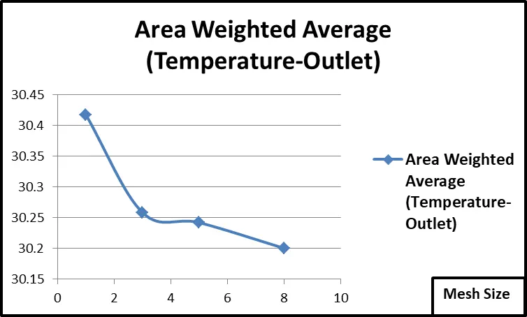
The standard deviation refers to how much the value varies away from the mean value. In other words, the standard deviation for temperatures at outlet must be close to zero for accurate results. The area weighted average function in ANSYS FLUENT 2021 R1 gives us the average temperature value of the selected region, here it is the outlet section. The analytical value for outlet temperature is 29.725⁰C as mentioned previously.

The solution for the 8e-3 mesh size converged at 178^th iteration.

The solution for the 5e-3 mesh size converged at 163^rd iteration.

The solution for the 3e-3 mesh size converged around 200^th iteration.

The solution for the 1e-3 mesh size converged at 130^th iteration (approximate time is 6 minutes for Intel(R) Core(TM) i7-8750H CPU @ 2.20GHz 2.21 GHz, 16.0 GB RAM).

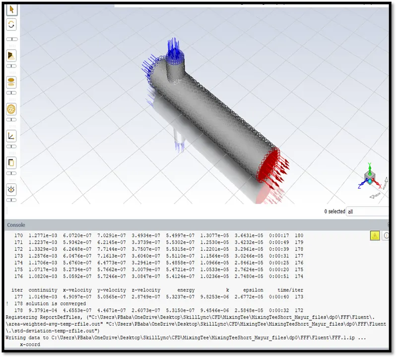
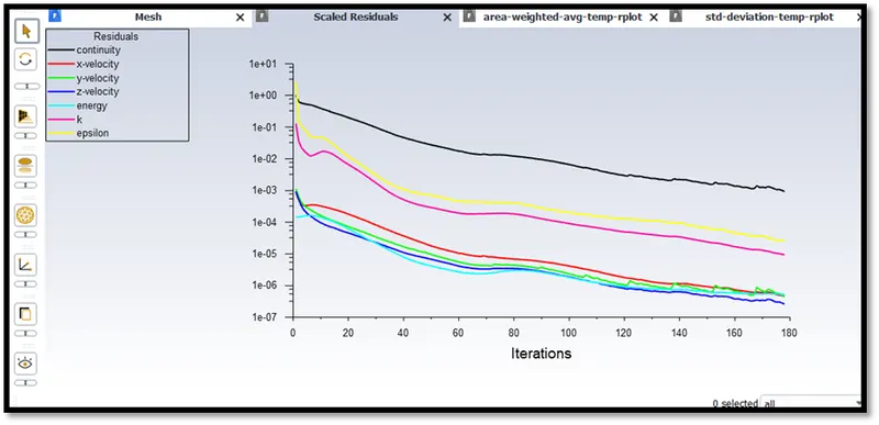
Iteration convergence and residual images for the 8e-3 mesh size simulation

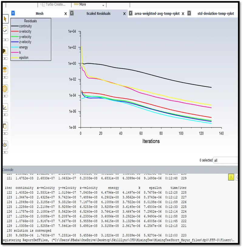
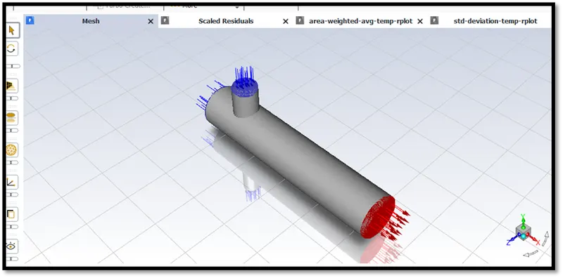
Iteration convergence and residual images for the 1e-3 mesh size simulation

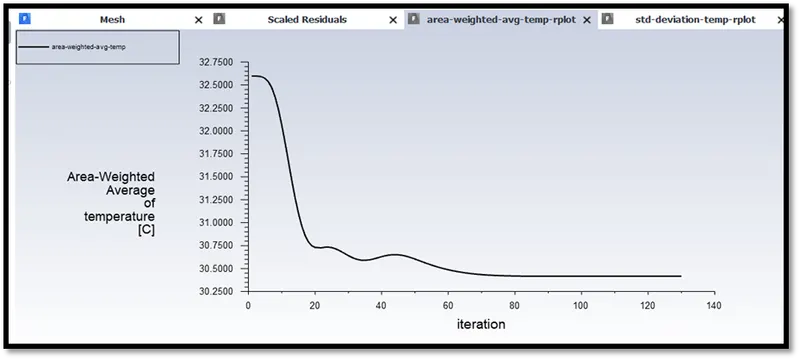
Area Weighted Average for the 1e-3 mesh size simulation

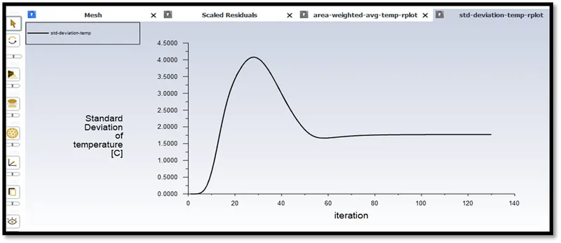
Standard deviation for the 1e-3 mesh size simulation

The standard deviation and area weighted average for different mesh sizes - coarse to fine i.e., from 8e-3 to 1e-3 at outlet, temperature, are given below.

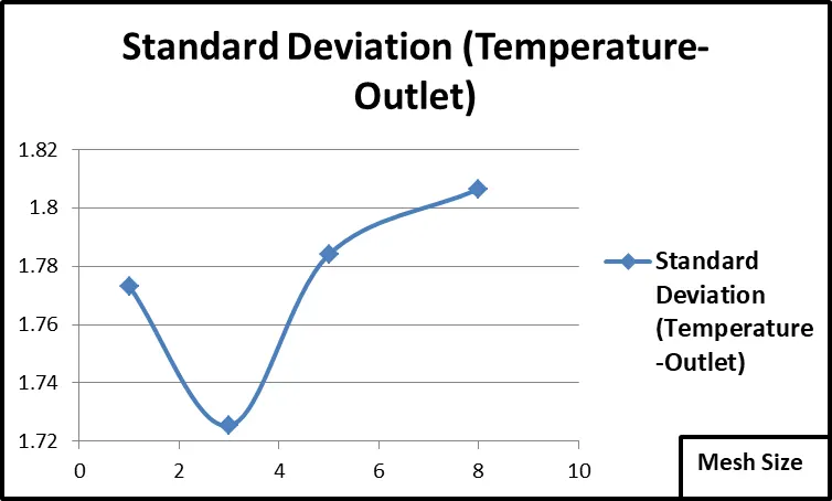
For standard deviation, the rate of change between the 1e-e and 3e-3 mesh size vary by 2.7284%. The rate of change between the 3e-e and 5e-3 mesh size vary by 3.3475%.

The rate of change between the 5e-e and 8e-3 mesh size vary by 1.25%.

For area weighted average - temperature at outlet, the rate of change between the 1e-e and 3e-3 mesh size vary by 0.52401%. The rate of change between the 3e-e and 5e-3 mesh size vary by 0.053487%. The rate of change between the 5e-e and 8e-3 mesh size vary by 0.1377246%.

The solver type is “pressure-based” for this particular steady flow problem, for both cases momentum ratios are checked for:

MOMENTUM RATIO	2	4
VELOCITIES (cold fluid-y)	6	12

The temperatures are kept at 36⁰C and 19⁰C for the hot and cold fluids at inlets 'x' and 'y' respectively for both cases.

RESULTS

The results show that the temperatures decrease after the mixing happens at both the inlets. The length of the horizontal pipe aft of the inter-section of the two inlet axis helps to enhance the mixing till the temperatures of the fluids are affected at outlet. These mainly depend on two main reasons:

• Velocities of the inlet fluids
• Temperatures of the inlet fluids

There can be a case study for the effect of variation of the mixing tee geometries, but that is not important for this report as both the geometries are same and do not vary for the change of momentum ratios, CASE ‘A’. Hence the two points mentioned above are of primary concern.

CASE ‘A’ Short Mixing Tee

Here, the velocities of the inlet fluids are checked for two points.

1. The velocity at the horizontal inlet is set lower than the vertical inlet fluid velocity but the temperature of the latter is relatively cooler. This temperature difference shows the effectiveness of the mixing within the volume extract or fluid domain.
2. The velocity for the horizontal inlet is at 3m/s and that of the vertical inlet pipe is set to 6m/s and also checked for 12 m/s. However the temperature of the hot fluid is 36⁰C and that of the cold fluid is 19⁰

CASE ‘B’ Long Mixing Tee

The inlet y velocity of the vertical pipe is checked for momentum ratios 2 and 4. Same points as mentioned for CASE ‘A’ are followed, only the geometry differs.

The velocity of the hot fluid is set to 3m/s for all cases.

The mesh size of 3e-3 is considered to get the output for CASE ‘A’ and CASE ’B’.

SHORT & LONG MIXING TEE

The mesh size of 3e-3 is chosen considering the time for solution being lesser than the 1e-3 mesh size as there is a rate of change value of only 2.72% and 0.52% for standard deviation and area weighted average of temperatures at outlet respectively between the mesh sizes for accurate results.

The solution converged at 158^th iteration for a momentum ratio of 4, short mixing tee and around 250^th iteration for the long mixing tee.

Momentum Ratio	CASE ‘A’		CASE ‘B’		Analytical results
	Standard Deviation (Temperature) (0C)	Area Weighted Average Temperature at Outlet (0C)	Standard Deviation (Temperature) (0C)	Area Weighted Average Temperature at Outlet (0C)
2	1.7253949	30.258168	0.99509484	30.372923	29.725 0C
4	1.0645817	27.630572	0.86496759	27.520129	30.18802

The values for the analytical calculations for the long mixing tee at MR=2,4

are:

Mass flow rate-y = A*V = 0.00025574199 m² * 6 m/s = 0.00153445194 m/s

Mass flow rate-x = A*V = 0.0009846037m² * 3 m/s = 0.0029538111

We get the T_mixture as 30.1880⁰C using the formula as stated previously, this is the analytical temperature at the outlet for the long mixing tee.

CASE A

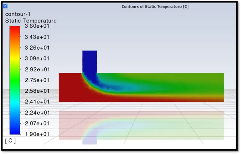
Temperature profile at mid-plane section – Short Mixing Tee MR=2

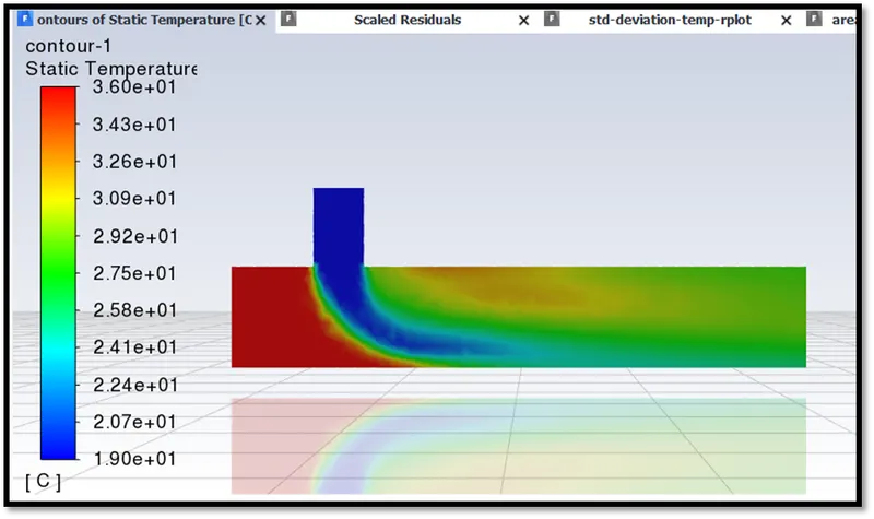
Temperature profile at mid-plane section – Short Mixing Tee MR=4

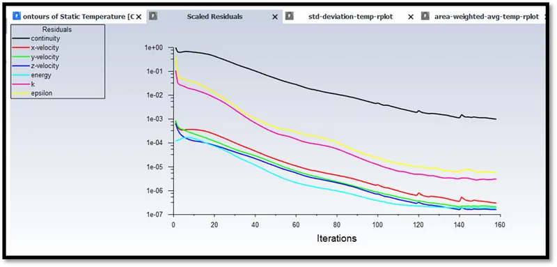
Residuals MR=4, short mixing tee

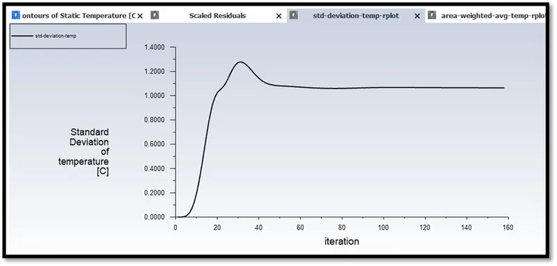
Std. Deviation MR=4, short mixing tee

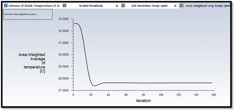
Area weighted avg. short mixing tee, MR=4

CASE ‘B’

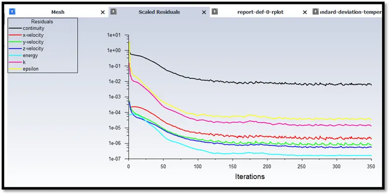
Scaled residuals for long mixing tee MR=2

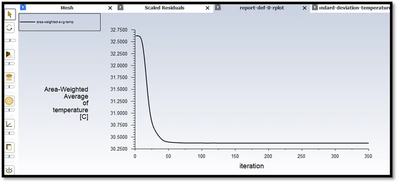
Area weighted average of CASE ‘B’, MR=2

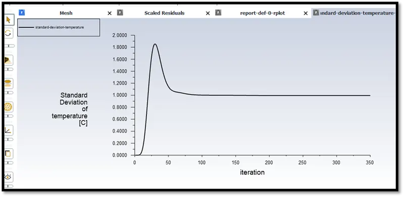
Standard deviation of CASE ‘B’, MR=2

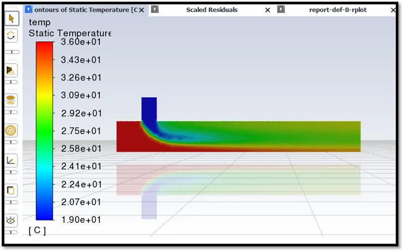
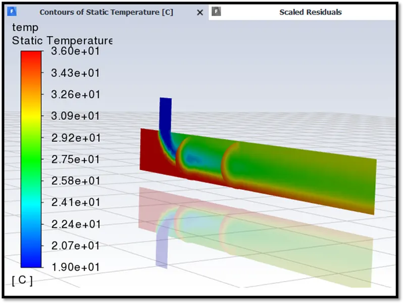
Temperature contour for long mixing tee, MR=2

CASE B ; MR=4

The solution converged around 180^th iteration. The scaled residuals, area weighted average, temperature contour and standard deviation plots are given below.

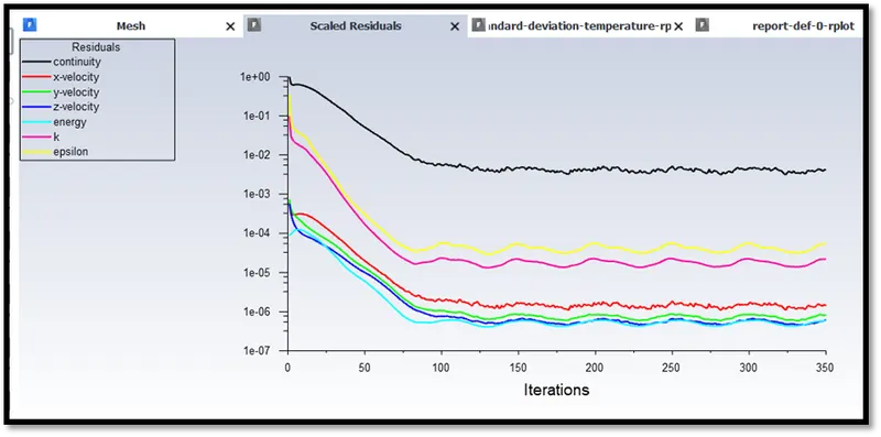
Scaled residuals for CASE ‘B’, MR=4

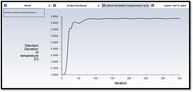
Standard deviation of temperature at outlet plot for CASE ‘B’, MR=4

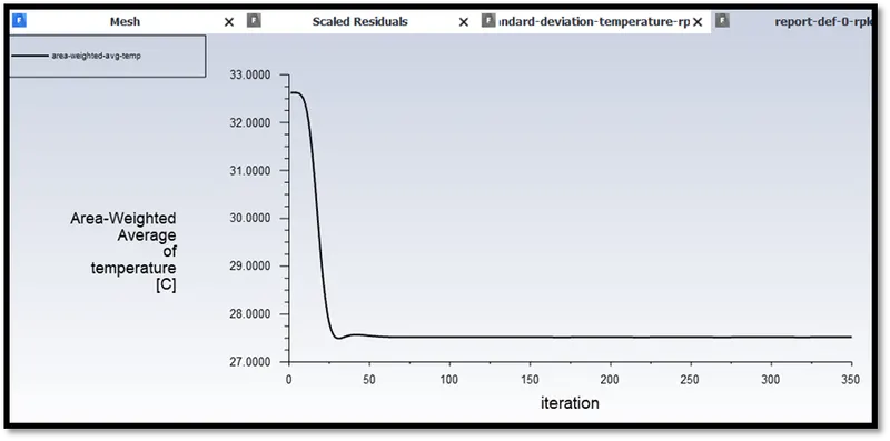
Area weighted average of temperature for CASE ‘B’, MR=4

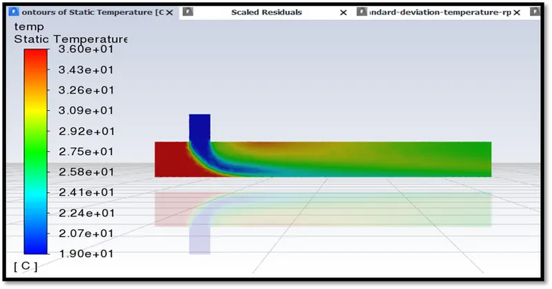
Temperature contour for CASE’B’, MR=4

The velocity contour plot for the long mixing tee for a momentum ratio = 2 and 4 are given below.

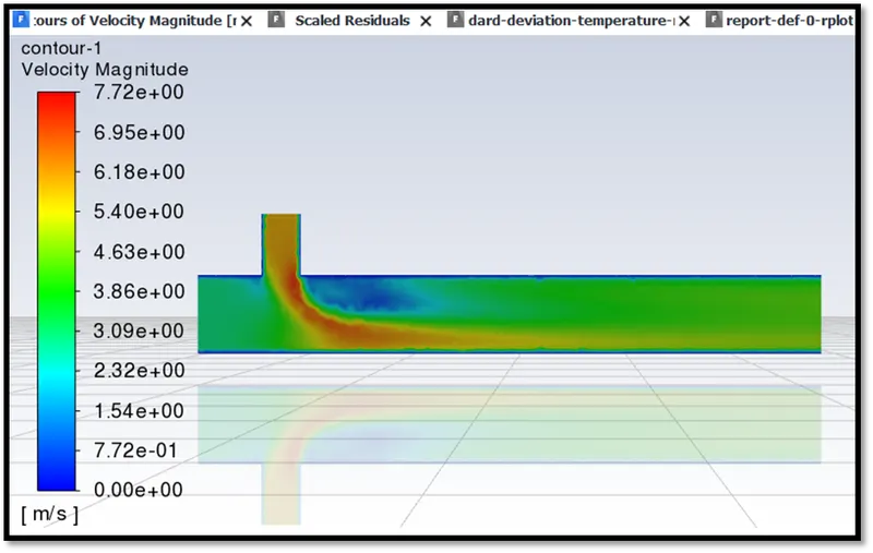
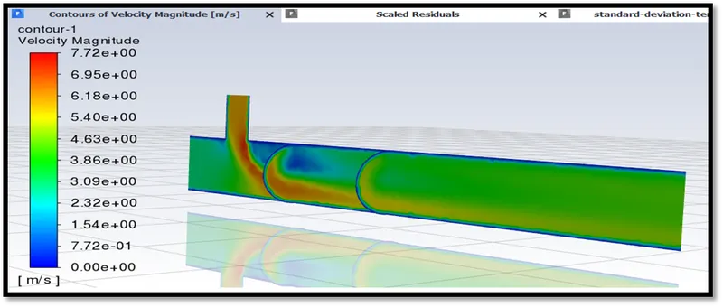
CASE B, MR=2

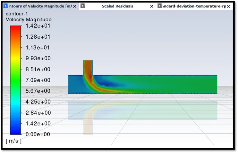
CASE B, MR=4

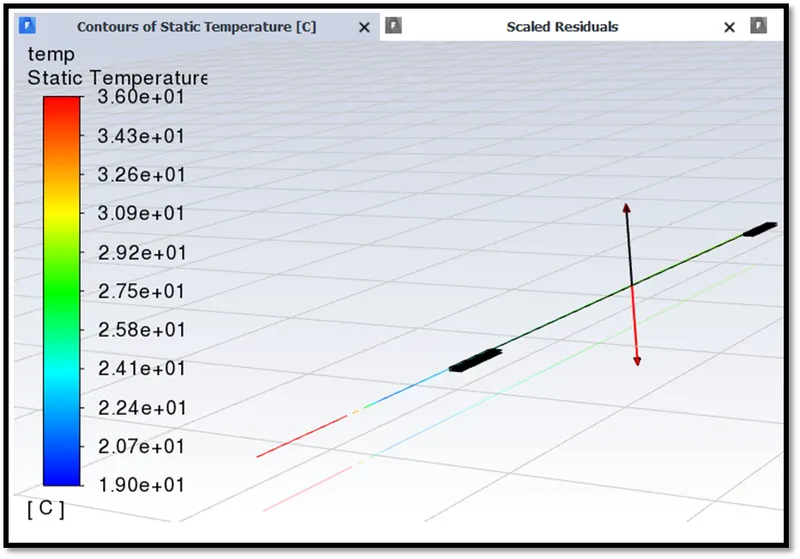
CASE B, MR=2 line temperature plot

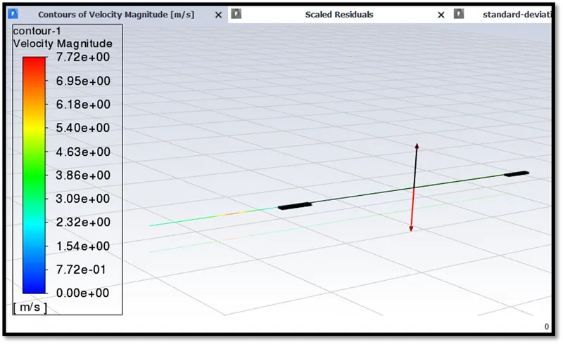
CASE B, MR=2 line velocity plot

The vertical lines are plotted at different x axis distance, followed by the chart of the temperature and velocity plots along the pipe flow direction.

This is for CASE ‘B’, long mixing tee for a momentum ratio = 2. (Hot fluid inlet = 3m/s and cold fluid inlet is 6 m/s).

The vertical lines are plotted for a distance of x = -0.02313m, 0.00745945m, 0.0664917m and 0.190995m (approx. 0.2m).

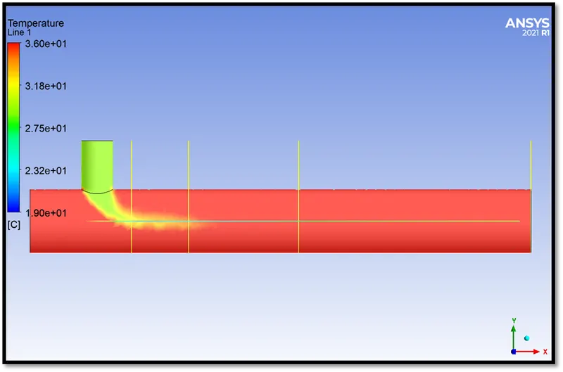
Temperature contour

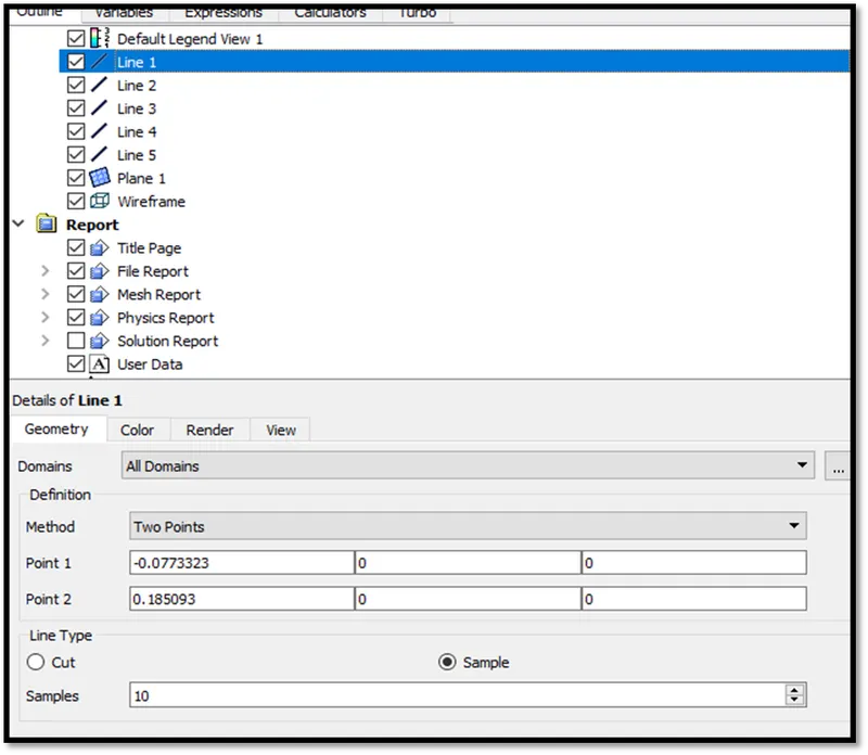
Line 1 x axis point values

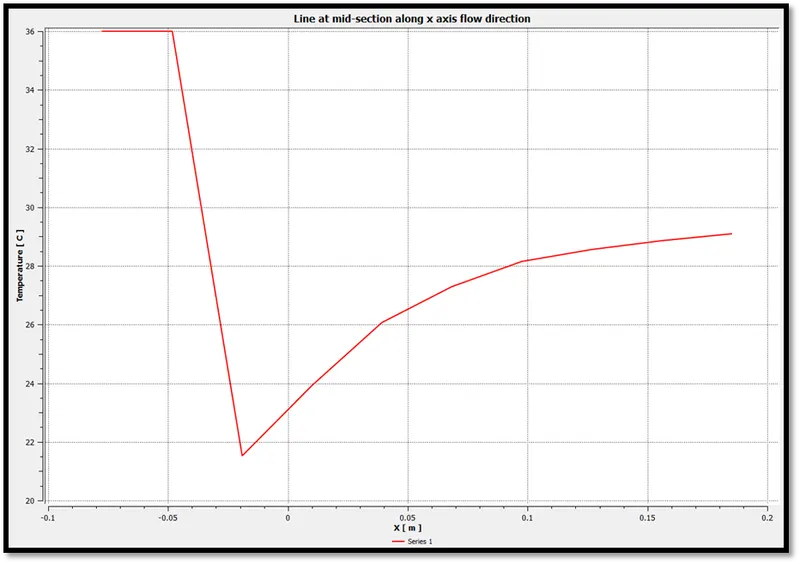
Horizontal line temperature plot – Line 1

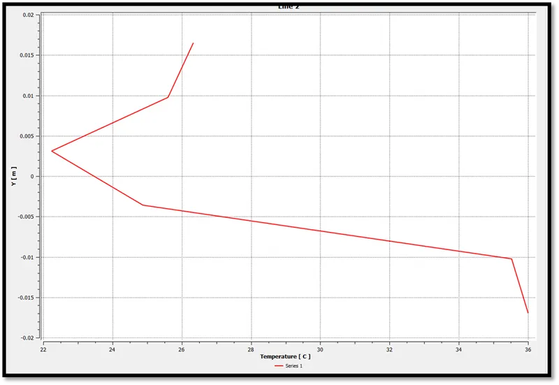
Line 2 – temperature plot

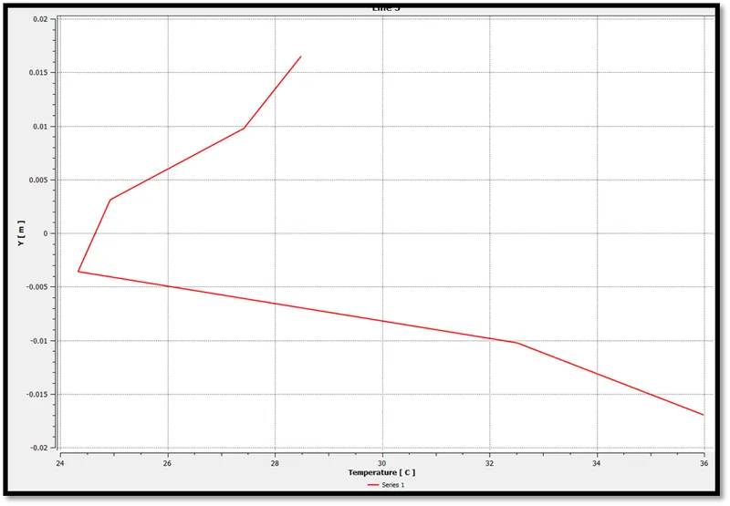
Line 3 – temperature plot

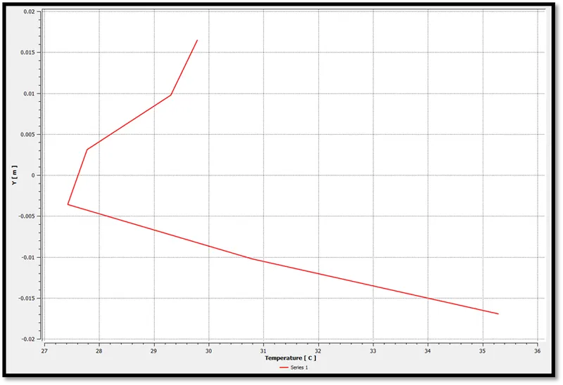
Line 4 – temperature plot

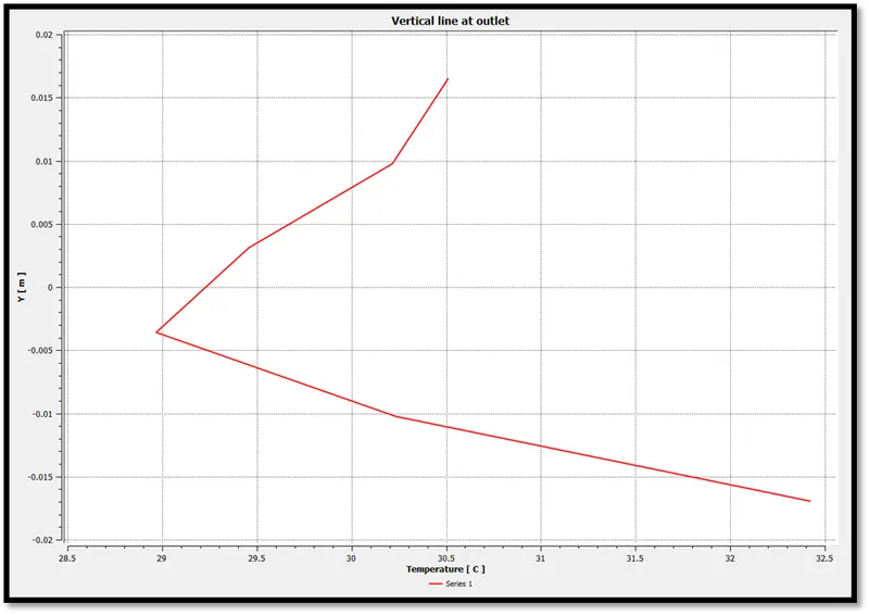
Line 5 – temperature plot

The temperature at outlet section varies rather asymmetrically. This is due to the placment of the inlet-y pipe for the cold fluid which intersects the hot fluid flow along x-axis. Thus the fluid has a pressure around the two inlets and the flow gets deviated to the bottom right near the outlet section. This gives us a temperature curve as shown above.

These are the 4 lines. Line 1 refers to the horizontal line along the x axis flow direction followed by the lines 2,3,4 and 5 for the vertical lines from the left of the axial flow direction. The velocity plots for the same are as follows.

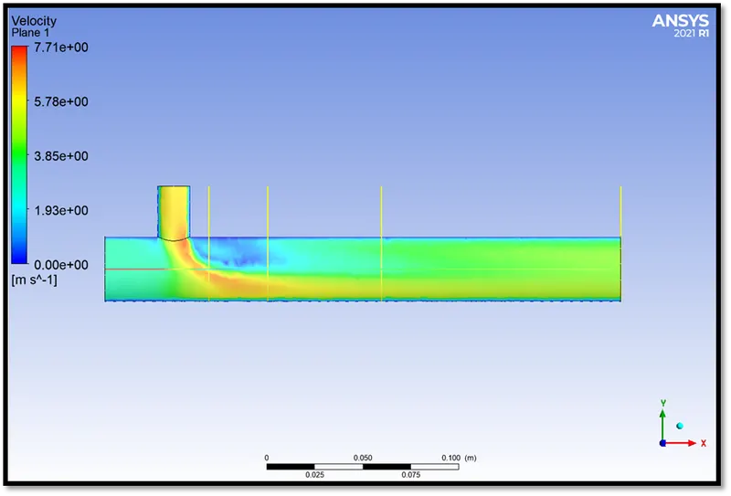
Velocity contour CASE ‘B’; MR=2

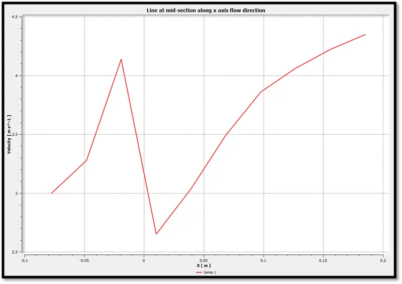
Horizontal Line 1 – velocity plot

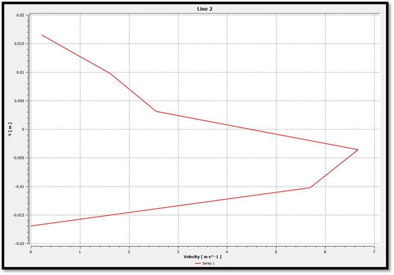
Line 2 – velocity plot

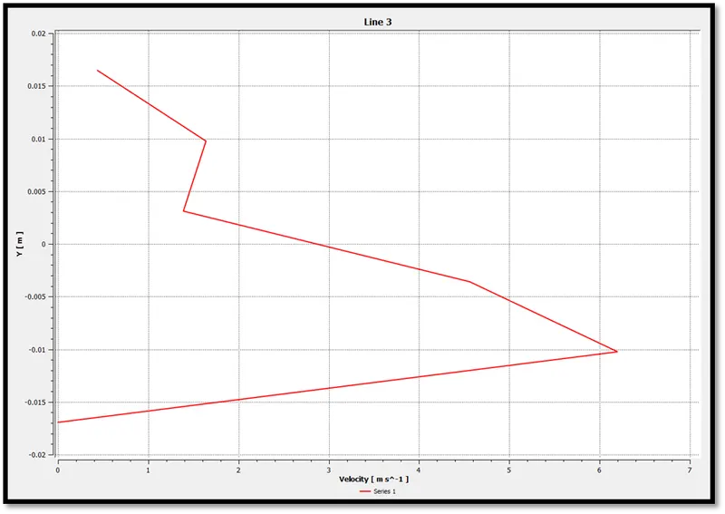
Line 3 – velocity plot

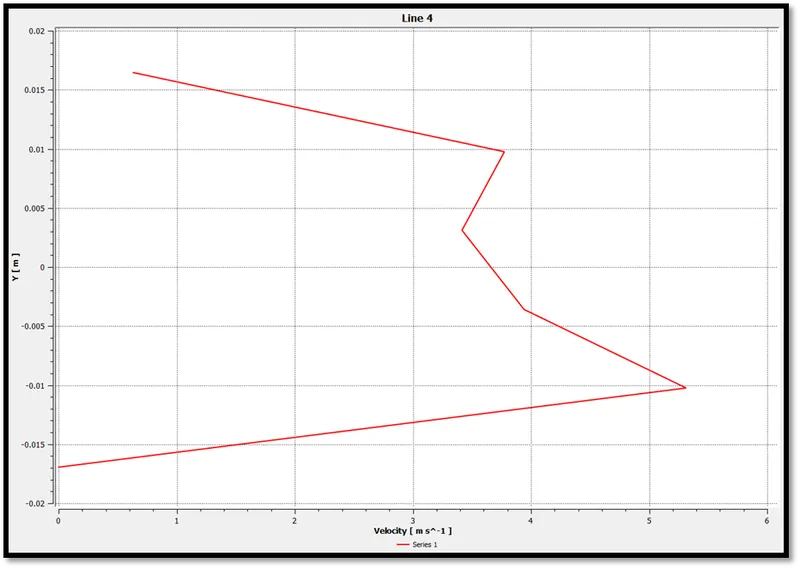
Line 4 – velocity plot

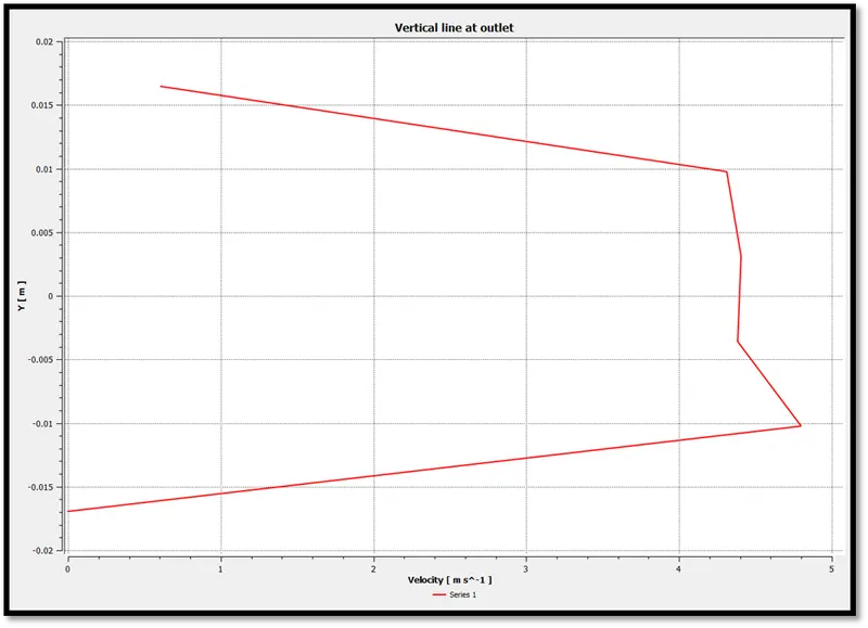
Line 5 at outlet – velocity plot

It can be noted that the mixing effectiveness is almost constant for most of the vertical section at the outlet for the long mixing tee for a momentum ratio of 2. The mixing effectiveness increases as the inlet fluid velocity increases thereby enhancing greater mixing effciency at the outlet region. Also the velocity will be lower due to the velocity gradient and shear wall stresses which occurs due to viscosity and friction near walls. Hence the effectiveness is noted mainly closer to the mid center points from inlet to outlet sections of the horizontal pipe.

Conclusion

The mixing tee problem can be checked for a variety of other parameters starting from the problem definition and change of geometry. The research gaps noted in this particular problem is the improper mixing effectiveness at the outlet section. This is satisfactory but can still be improved. The temperature curve does not provide uniform values at outlet for the k-e turbulence model. To satisfy the condition, the boundary conditions can be checked for another inlet in the y direction close to the x-axis mid section or reduction of coolant fluid temperature to a greater extent. The solution can be enhanced and achieved by availing the lengthening of the x-axis mixing tee pipe. However the consideration of conjugate heat transfer to capture an even more realistic problem-solution can be worked upon with different solid materials of high heat transfers rates.

The 3e-3 mesh size is chosen for the simulation of both the short and long mixing tee analysis as the solution converges and values close to the analytical results are obtained with less than 5% error.

Case ‘A’ depicts the short mixing tee flow problem. The standard deviation for this case vary by 47.37% between momentum ratios 2 and 4. The area weighted average has a difference percentage of 9.078% between the two sub cases i.e., MR=2,4.

For the long mixing tee problem, case ‘B’, the standard deviation varies by 13.9917% between momentum ratios 2 and 4. The area weighted average has a difference percentage of 9.8554% between the two sub cases i.e., MR=2,4.

This proves that as the length of the horizontal pipe increases the mixing efficiency increases, hence a better standard deviation (close to zero) value can be obtained at the outlet section in comparison to the short mixing tee problem.