Report on Week 2 Challenge : Pressure Valve Meshing

B A Mayur

Aim: Surface mesh of a valve by performing a geometry clean up and generating faces where necessary.

Theory:

Every part must be closed to perform a meshing operation. Hence the single cons (red edges shared with one surface), double cons (yellow edges - shared with two surfaces) and the triple cons (blue edges – shared with three surfaces) are to be closed.

Procedure:

Import pressure valve model and the steps are followed towards meshing the model after topo clean up and stringent geometry checks.

The pressure valve model is first imported into the ANSA environment (v23.1.0).

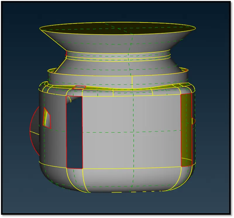
Fig: Pressure valve model (Shadow option enabled)

We can see that the geometry has a few patches i.e. it is not closed. Hence we can select the faces -> New option to fix the surface.

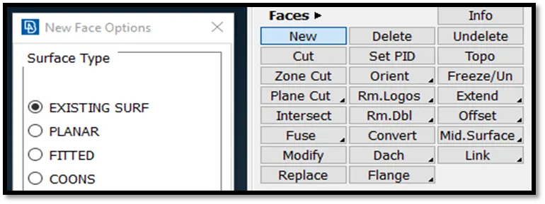
Fig: Existing Surface option

The cons (edges) are to be selected to obtain a closed surface. The edges selected shows that we are interested to tweak that particular surface followed by the middle click (mouse wheel button -3) for confirming the selections.

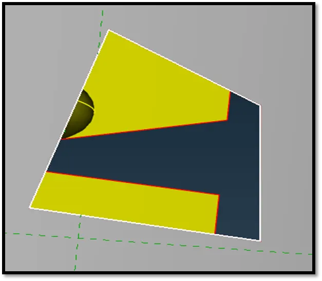
Fig: Edges (cons) are selected

The meshing environment now asks for the face to be selected to get the new surface. This can be done by selecting the surface with the help of cross hatches (in green). The surface will be created.

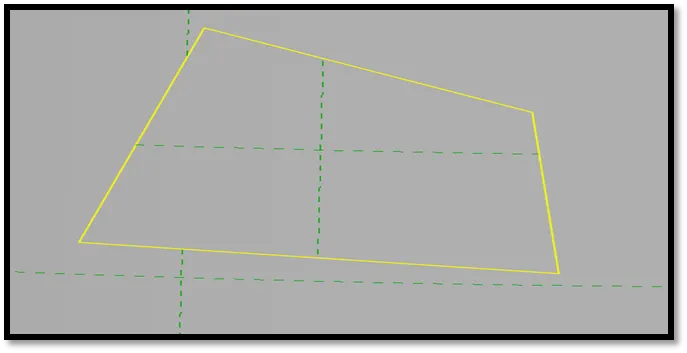
Fig: New surface created

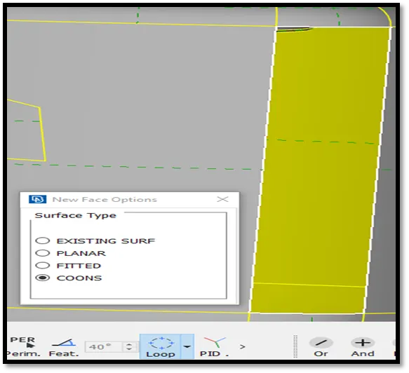
Fig: Coons operation

The same operation outcome can be achieved by using the ‘Coons’ function and enabling the ‘Loop’ option. This was we can select only one con and the surrounding edges (in loop) are auto-selected. The mouse button 3 is pressed to confirm the new surface.

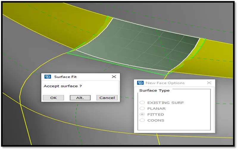
Fig: Fitted option

The ‘Fitted’ algorithm works the same way as ‘Coons’ algorithm. The con is selected and the loop option enables selection of the edges in loop. The ‘Alt.’ option shows the alternate surface that can also be created and the new surface is created by selected ‘OK’.

The ‘PLANAR’ algorithm can be used to patch the surface pertaining to a particular plane only.

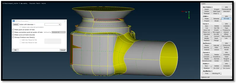
Fig: Fill Hole option

By using the CONS -> ‘Fill Hole’ option, we can select the circumference of the hole and middle click to complete generation of the surface.

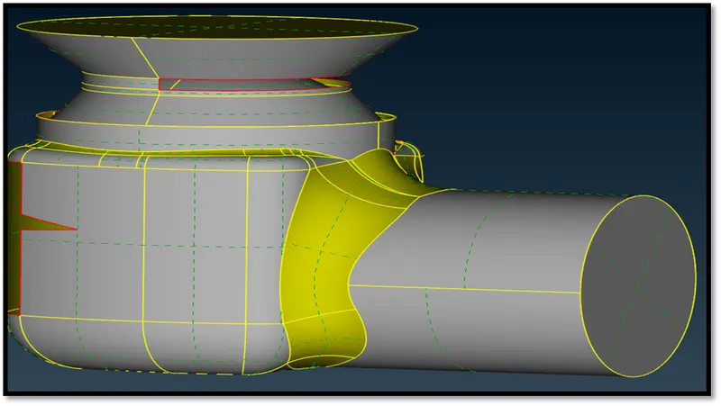
Fig: Hole is filled with a surface

The ‘FITTED’ option is used to fill the triangle patch by individually selecting the entity (edge) instead of ‘Loop’ option.

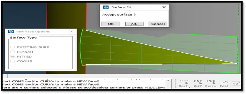
Fig: ENT option to select entity (edges) – FITTED Option

Also the rectangular is filled using the CONS -> ‘FILL HOLE’ option.

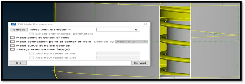
Fig: Fill Hole option to fill rectangular patch

The other surfaces are filled by using a combination of fill holes and new faces option. Fill holes option can be used to select multiple patches to create surfaces. ANSA allows us to see the edged marked in red (single cons or open surfaces) by holding the Ctrl + Shift keys.

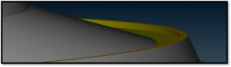
Fig: Surface missing

We can see that there is no cross hatches (in green) present as the surface is missing which needs to be created. Once a surface is created, the red edges will turn to yellow (double cons). We can perform the operatio using the ‘COONS’ option. While selecting the edges, we must make use of the wireframe mode to verify that the lengths of the edges are same. This is only to make sure that the selections of the single cons are proper.

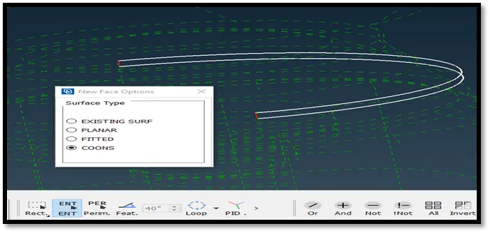
Fig: Selection of single cons

If the selected cons are not of same lengths, we may not be able to get the required surface perfectly (uneven surface). For the other two cons at the ends of the semi circumference, the cons are to be clicked twice in the wireframe mode. The new surface will thus be created (cross hatches can be seen).

The same procedure is followed to also fill the vertical surface-patch at the bottom region of the pressure valve.

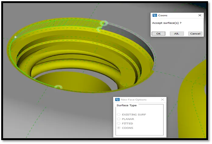
Fig: Vertical surface created

The edged are selected such that they are of same lengths to create the vertical surface fill. This is done twice to complete the surface fill of the whole patch. The geometry is closed by creating a surface for volume meshing by selecting the newly obtained double cons. This way, triple cons will be obtained at the circumference of the surface.

A geometry check is performed to obtain the status of the geometry for a positive feedback.

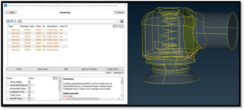
Fig: Geometry check

This completes the topo clean-up by eliminating all the single cons. For the CFD simulation, we need a closed model which is now feasible. However a few other geometry checks have to be addressed.

There will be surfaces created by the CAD department to capture simulation results effectively which may give space to uneven surfaces. These surfaces must be checked if the mesh element size fits within the space. Hence to remove such spaces we use the ‘CUT’ option.

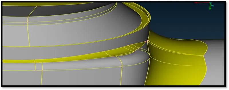
Fig: Small unwanted surface

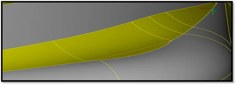
Fig: Line removed (orange colour shows the line was present but now removed)

Similarly lines very near to each other or unwanted lines can be removed to accommodate the mesh element sizes greater than the distance between the lines.

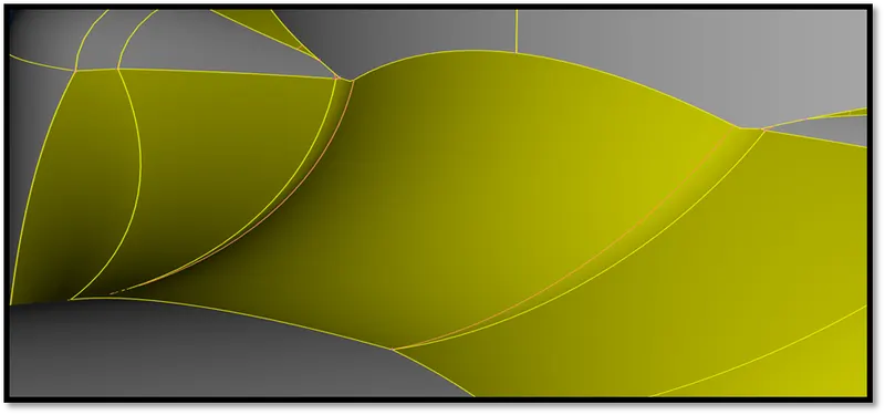
Fig: Lines removed are indicated in orange colour

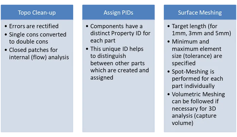
Now new PIDs (property ID) are created and assigned to the assembly which helps to set boundary conditions in the simulation domain.

Now the PIDs are assigned to the required cross-hatch.

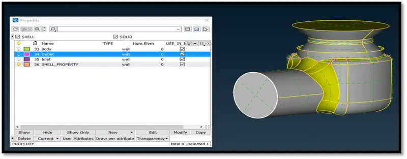
Fig: Assign Outlet to required cross-hatch

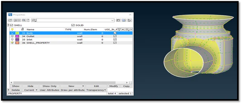
Fig: PID assigned to body by isolating it using the ‘OR’ and PID region selection option

To select a component, the ‘PID region’ option or the ‘Entity’ option is used to select the part and assign a PID. It can also be completed by hiding the other already assigned parts to make the component to be assigned visible and assign the respective PID for the part.

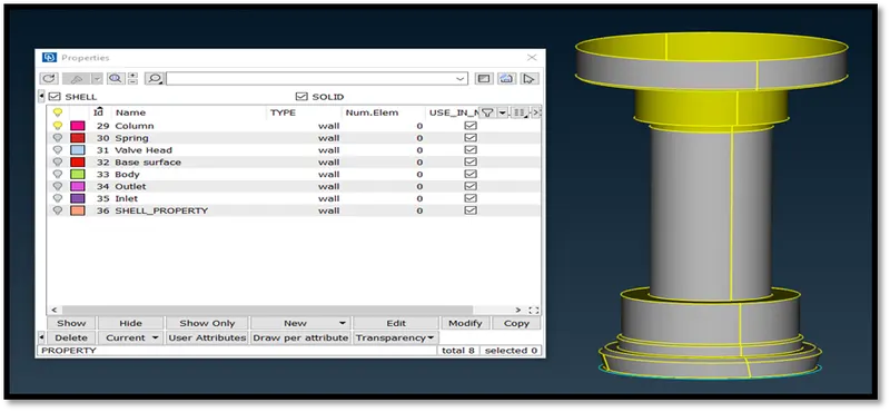
Fig: Column PID assigned

This way all PIDs are assigned to parts using the tools.

Now we can continue towards the meshing operation of each component. Three cases are made for different mesh sizes i.e., 1mm, 3mm and 5mm mesh element size lengths.

The mesh parameters, quality criteria, perimeter and macros options are tweaked accordingly.

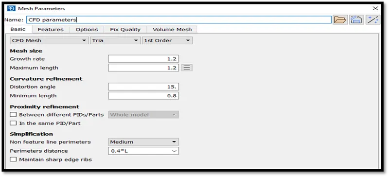
Fig: Mesh Parameters

The CFD mesh option is chosen to perform the operation for 1mm mesh element size (target size). Similarly, the quality criteria minimum and maximum length values are set with a tolerance of 0.2mm i.e., 0.8mm and 1.2mm. The mesh element is set to ‘Tria’ to obtain triangular mesh elements.

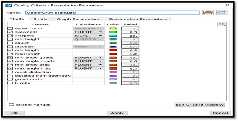
Fig: Mesh Quality Criteria

We can now start to perform the mesh operation using the Spot Mesh option and selecting the required component to mesh.

Learning Outcomes:

The steps followed has supported for a clear description to perform a neat topo-clean-up followed by meshing of individual components. The use of the tools provided by ANSA helps to ease the operations and procedure to a specified target mesh length size for simulations.

Result:

The outlet is meshed first and the method used is to individually penetrate through all the parts by meshing them individually for precision.

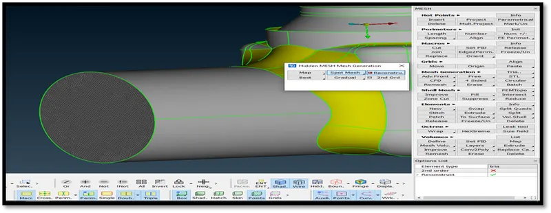
Fig: Outlet mesh

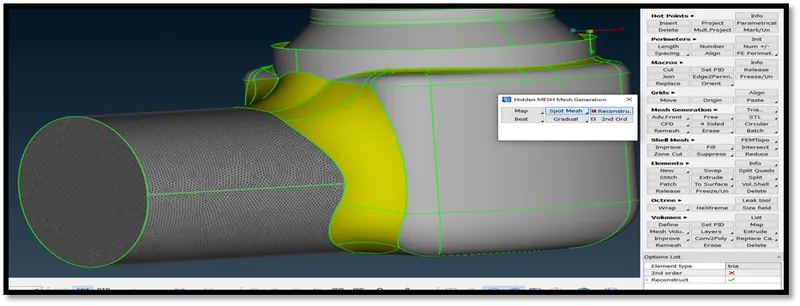
Fig: Neighbouring component is selected and mesh operation performed for 1mm

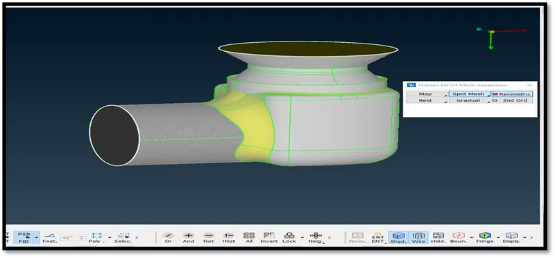
Fig: Body selected using the PID option selection method

The PID is selected to mesh the body and mouse button 3 is pressed to confirm the operation again.

The mesh is obtained as shown in the below figure.

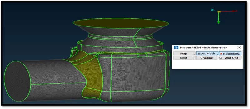
Fig: Mesh obtained for the selection

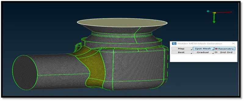
Fig: The top portion (inlet) is selected and meshed

The base portion is meshed by using ‘ShowOnly’ option from the properties-PID menu.

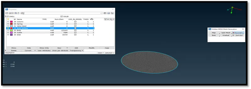
Fig: Spot-Mesh -> Visible

This option (SpotMesh - Visible) meshes all components shown in the graphics viewer. Now the body, base surface, inlet and outlet portions have been meshed completely.

The components yet to be meshed are made visible and meshed using the same way. We obtain a completely meshed assembly by following these steps as shown in the below figures.

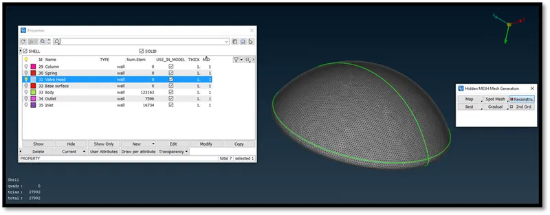
Fig: Valve head mesh

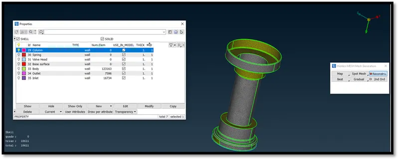
Fig: Column Mesh

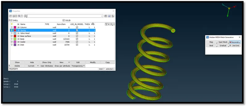
Fig: Spring Mesh

For the pressure valve, the mesh quality as seen can be improvised to a finer mesh if necessary. Also the spring component has a small diameter (cross-section) already. Therefore the mesh target length must be lower than circumference geometry dimensions so that the mesh can fit in.

Conclusion:

The mesh of the assembly is obtained by following these steps.

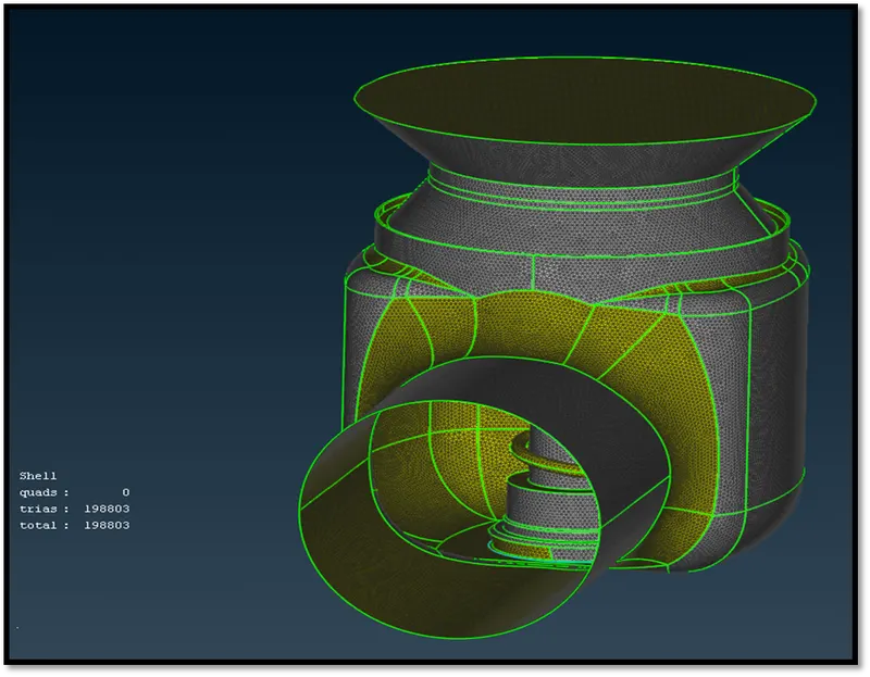
Fig: Full body mesh (1mm)

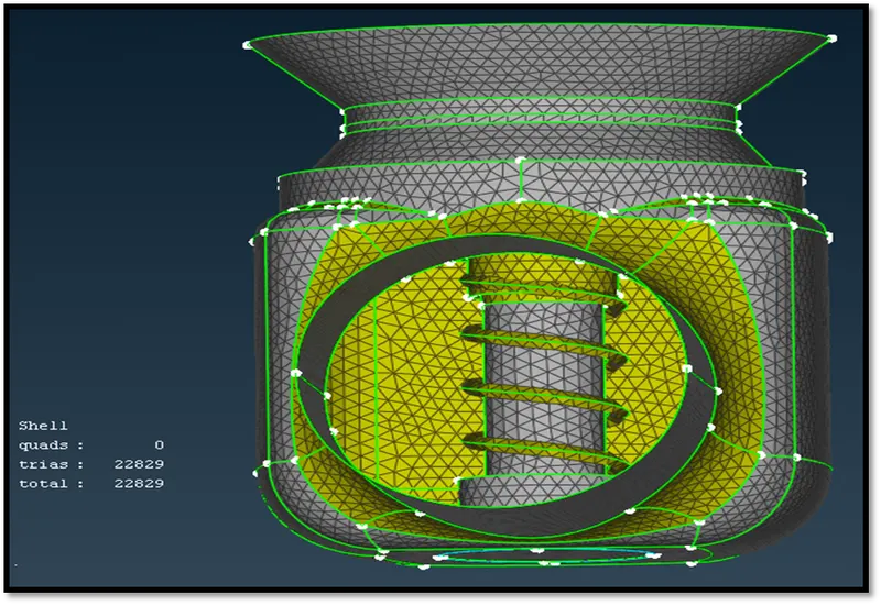
Fig: Full body mesh (3mm)

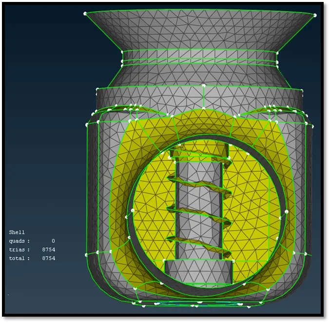
Fig: Full body mesh (5mm)

The table below shows the number of tria elements obtained for each component at different mesh sizes.

Part	Number of elements
Target length size	1mm	3mm	5mm
Inlet	16734	1878	676
Outlet	7596	786	298
Body	123163	13999	5254
Valve Head	27992	3154	1148
Base Surface	2345	255	106
Spring	9948	1276	594
Column	18621	2267	976

For the 5mm target size a minimum length of 3mm and maximum length of 6mm was specified. Yet the mesh of the spring looks inaccurate as the mesh element diameter seems to be greater than the distance of spring diameter at some regions. It is better to use a 3mm mesh element size for the spring. The calculation time will be quick for the 5mm mesh target length but the results cannot be better than 3mm mesh target size as it does not cover the regions completely with a coarse mesh. The 1mm mesh target size will give accurate results as it is finer with more calculation time per mesh block/ discretization.