Week 9 - Parametric study on Gate valve.

Introduction to GUI based CFD using ANSYS Fluent

Gate valve Simulation – Parametric Study - Report

B A Mayur

INTRODUCTION

A gate valve is a control valve which is used to permit the fluid flow through a pipe. Depending on the level of the gate valve position, the flow can be allowed to fully flow through the pipe or the flow can be completely shut off in closed position. Usually it is installed in pipes carrying non-flammable fluids like oil, water or light grease.

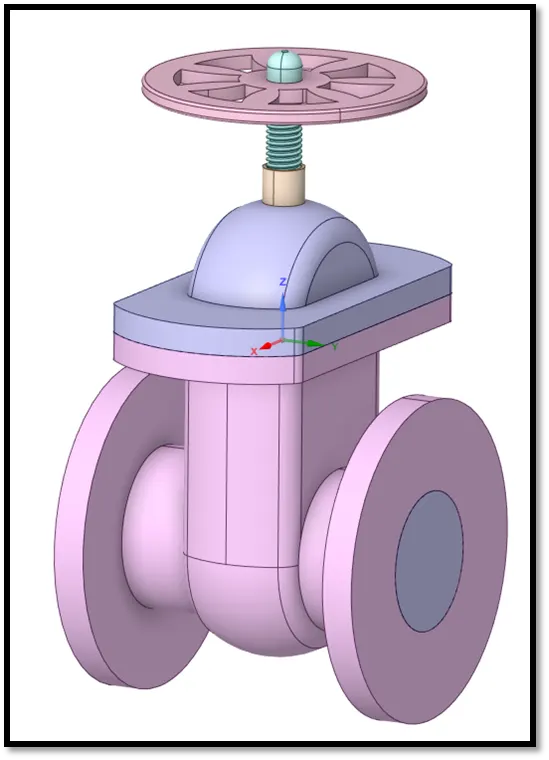
Fig: Gate Valve Model

AIM

• To analyze flow through a gate valve.
• Parametric study to analyze the mass flow rate at the outlet of the gate valve though different levels of lift of the gate disc.

THEORY OF THE PROBLEM

The gate valve consists of a hand wheel, a spindle that is connected to the gate disc which is enclosed by the bottom valve body. The hand wheel and spindle together control the level of the gate disc. This allows the passage of the fluid mass flow rate controlled by the height (level) of the raised gate disc within the gate valve. The mass flow rate is checked for different heights raised.

GOVERNING EQUATIONS AND OTHER SUPPORTING EQUATIONS

The conservation of mass, momentum and energy equations are used to calculate the problem and validate the analysis.

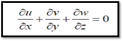
Conservation of mass equation:

Conservation of momentum equation:

Conservation of energy equation:

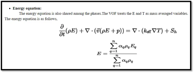
However, the energy equation is not solved for the simulation as thermal parameters are not used to set up the boundary conditions.

Reynolds Number (Re):

Where ‘ρ’ is the density in kg/m³, ‘v’ is the velocity in m/s, ‘D’ is the diameter of the cylinder in meter and ‘μ’ is the dynamic viscosity of the fluid in N/m².

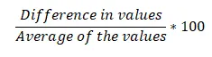
The formula for difference percentage is:

Bernoulli’s Principle Formula:

The Bernoulli equation is considered the statement of the energy conservation for the fluids that flow. This is considered to be the qualitative behaviour that lowers the pressure in the regions with high velocities. This is termed as the Bernoulli effect.

Problem statement:

The mass flow rates at outlet for various levels of gate disc heights are checked. This causes variation in the velocity and mass flow rate at outlet for different levels of gate disc openings. A parametric study reveals the effectiveness of automating the gate disc height within the body/casing of the gate valve. The fluid domain is extracted for a sufficient length in the fluid flow to maintain equilibrium between inlet and outlet.

SOLVING AND MODELING APPROACH

A few images show the dimension in front and right planes of the gate valve.

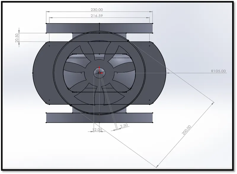
Fig: Front plane View

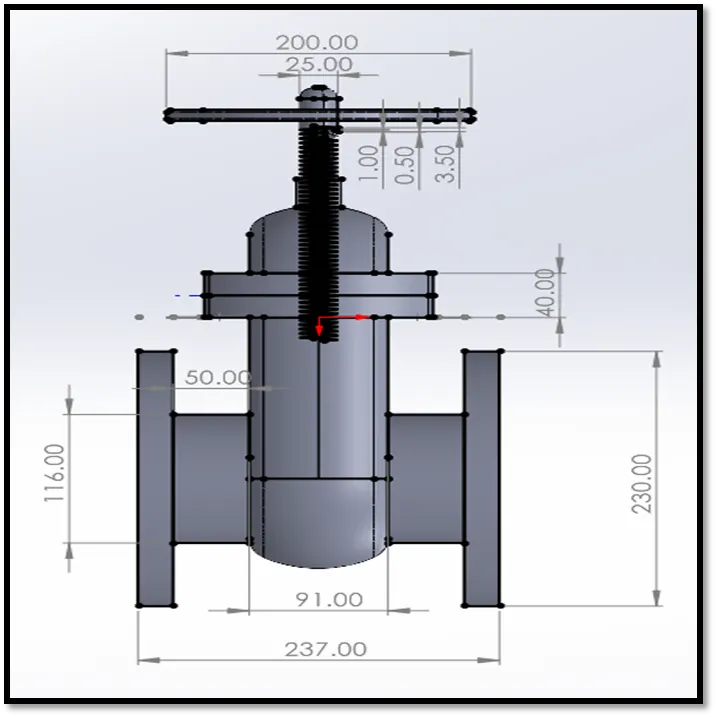
Fig: Right Plane View

Firstly, the design geometry is imported into SpaceClaim (drag and drop file into SpaceClaim environment). The bottom body and bonnet are hidden to make the gate disc, spindle and hand wheel combination visible for selection. The ‘Move’ tool is used to move the gate disk in Z direction, upwards by 10mm.

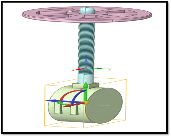
Fig: Spindle raised by 10mm

Since we want to model the parametric study of the mass flow rate at outlet which depends on the gate disc level/height raised, we create a ‘New Parameter’ under ‘Groups’ option. Fluent makes the Z direction (disc level in mm) of the gate disc as a new parameter which can be automated in the WorkBench environment.

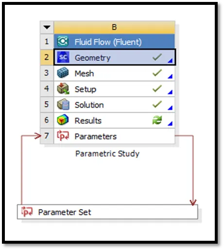
Fig: Parameter set for gate disc height

A volume extract is made under the ‘Prepare’ option in SpaceClaim. The volume extract is extended using the ‘Pull’ tool to facilitate the simulation of the fluid flow in the pipe. A length of 800 mm on either sides (inlet and outlet) will be sufficient to analyze the fluid flow domain.

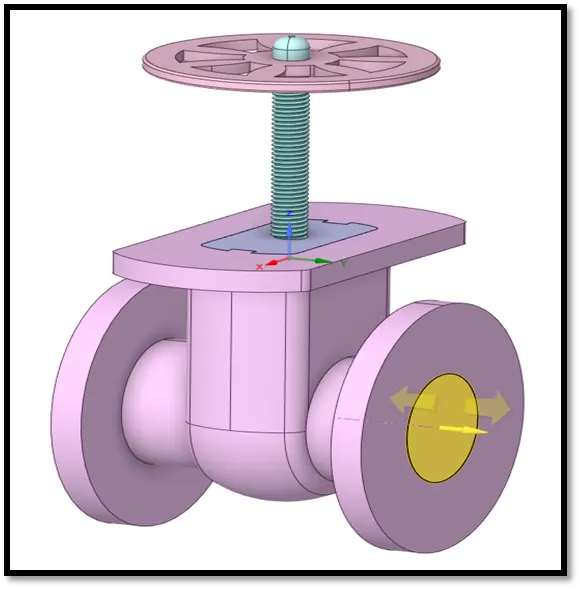
Fig: Volume extract is extended by 800mm on either side (fluid flow inlet-outlet)

This volume extract is needed for the parametric study and the solid bodies are suppressed for physics are they are not used for the simulation or in the mesh environment.

A base line mesh is generated for the volume extract and updated into the Fluent environment for pre-possessor settings and solving approach.

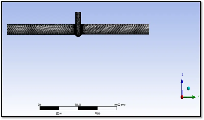
Fig: Base mesh

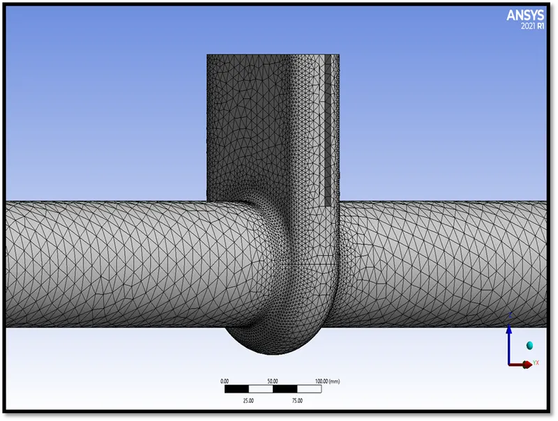
Fig: Mesh View of the model

Below is an image of the mesh details.

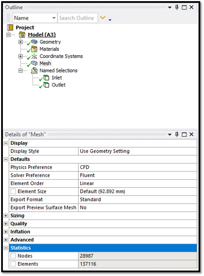
Fig: Named Selections and Mesh Details

The inlet and outlet named selections are made in the meshing environment to set up the boundary conditions. The base line mesh element size has produced 28987 nodes and 137116 elements.

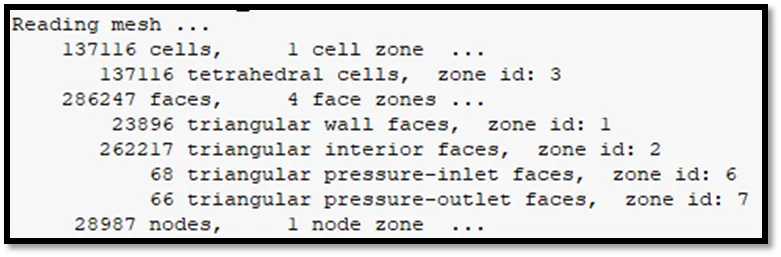
Fig: Mesh details

TURBULENCE MODELS

The turbulence model helps to specify the correct model needed for the simulation. A realizable k-e turbulence model is used to perform the simulation with scalable wall functions. The y+ value is greater than 11.126 irrespective of the level of near wall grid refinement. This value of y+ marks the intersection of the linear and logarithmic velocity profiles. In the realizable k–ε model, a non-constant value for dynamic viscosity coefficient (Cµ) is considered. It provides improved predictions for the spreading rate of both planar and round jets by considering a new formulation for the turbulent viscosity.

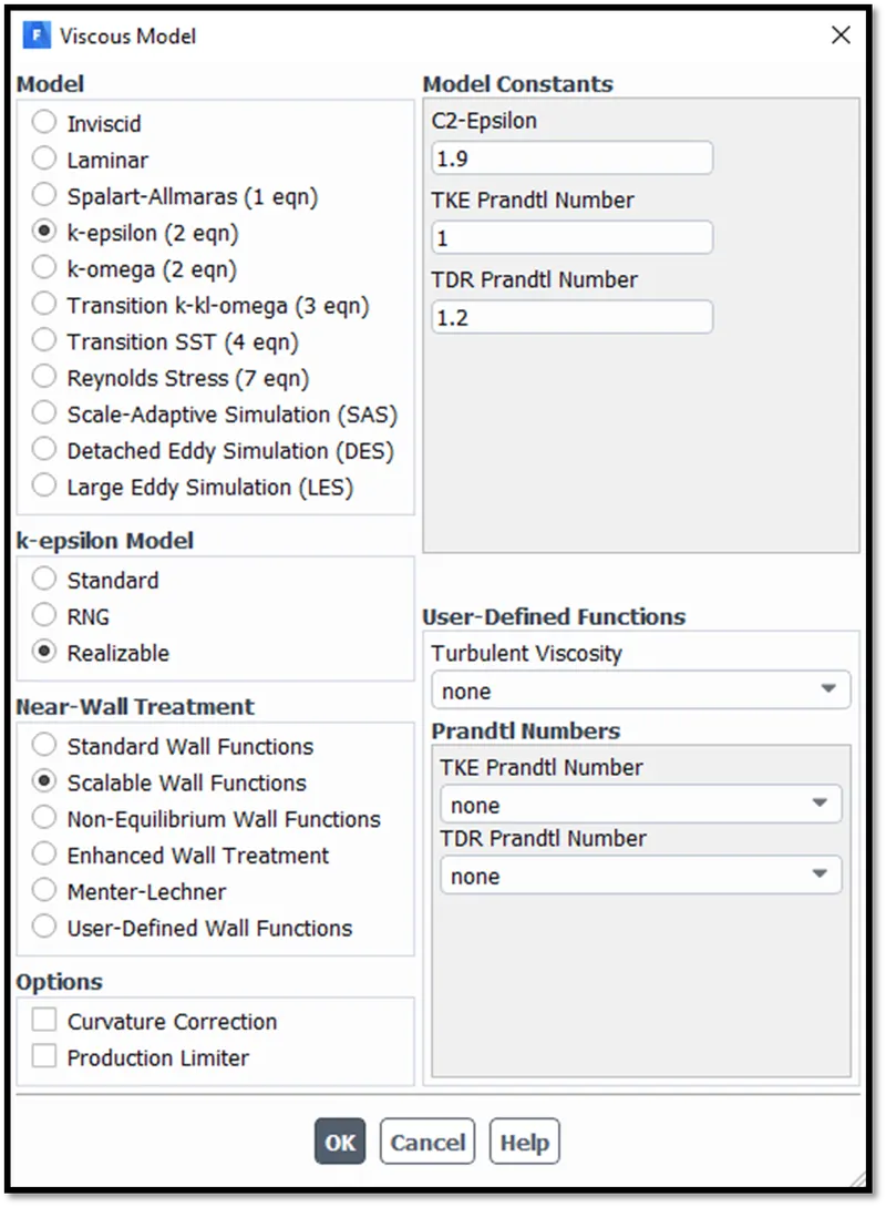
Fig: Turbulence Model

PRE-PROCESSING AND SOLVER SETTINGS

The simulation is performed using a pressure based solver with a steady state approach as we are interested in the end state results and not the values during the operation at intermittent levels which otherwise is a transient or time dependent simulation. The pressure based solver helps to consider an incompressible, low speed flows.

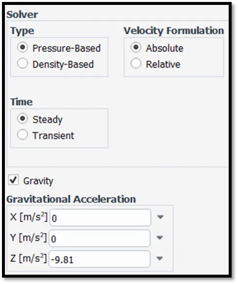
Fig: Solver Settings

The gravity term is enabled as 9.81m/s² in the negative Z direction to the model.

The fluid material is specified to water – liquid which is assigned/simulated under the volume extract for the analysis. The solid is specified as aluminum but not used anywhere in the simulation otherwise, also the default fluid material ‘air’ is deleted to avoid any mix-ups with setting up material properties.

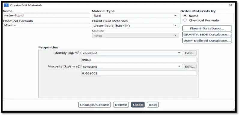
Fig: Materials - Fluid

The inlet type is set to a pressure based inlet and guage pressure is specified as 10Pa for the fluid flow.

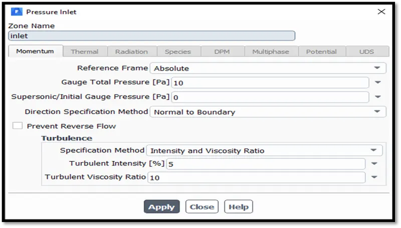
Fig: Inlet boundary condition

We can initialize the reference value computed from inlet. Here the velocity shown can be used to calculate the Reynolds number, which certainly gives a value lesser than 2000 i.e., in the laminar regime. Hence the k-e turbulence viscous model can be chosen for the simulation.

A velocity of 0.1415488m/s is seen. Using the Reynolds number formula, a value of 14087.1398, diameter of pipe is 100mm.

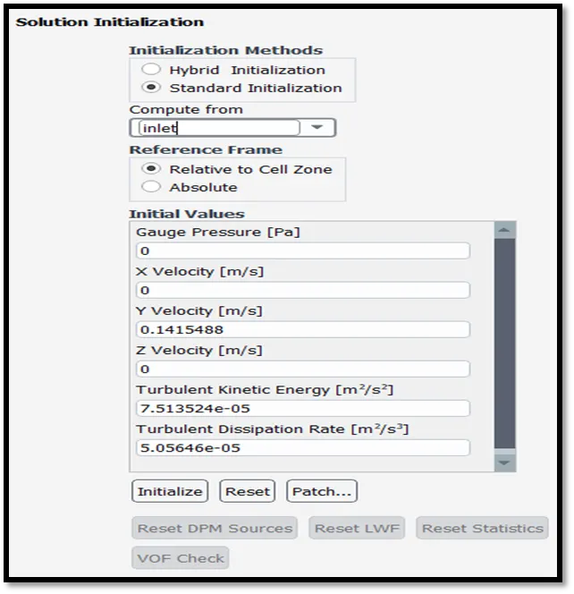
Fig: Solution Initialisation

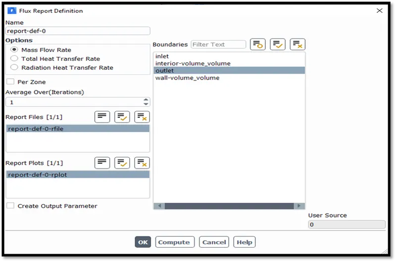
Fig: Flux Report Created

A new flux report for mass flow rate at outlet is created to obtain values which is printed to console and plot reported. A mid-plane is created to view the velocity contour and solution animation file before the calculation is performed.

As the gate disc height is parameterized, a new label called parameter as shown in the image previously helps to set up different gate disc levels to obtain results of the mass flow rate. The mass flow rates will be negative values depicting that the flow is getting out of the volume extract at outlet section of the fluid domain. 250 iterations were specified and the scaled residuals are shown for iterations till convergence is obtained.

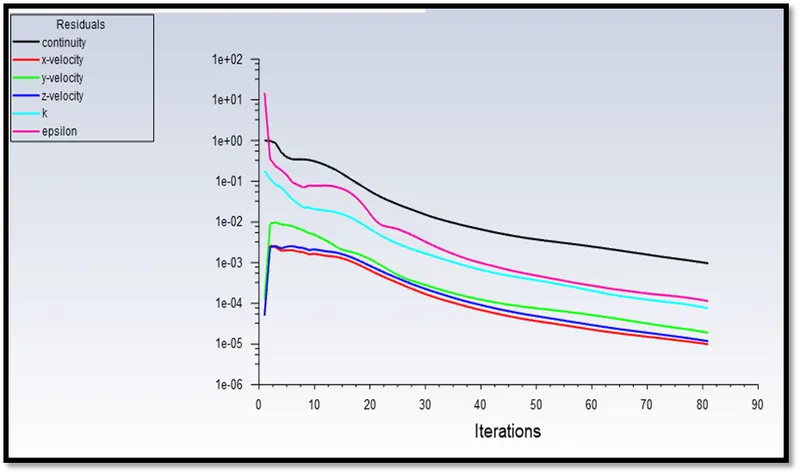
Fig: Scaled Residual plot for 10mm disc height

Various design points for the disc height were mentioned and calculation updated for all design points under the parameters option.

RESULTS

The mass flow rate for 10mm disc height is as shown in the image below.

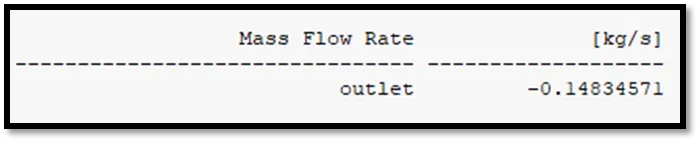
Fig: Mass flow rate – disc height raised by 10mm

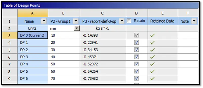
Fig: Table of Design Points

The retain option is checked to obtain the mass flow rate values for all design points. The ‘set as current’ option enables to view the Fluent Setup of the required design point simulation. A maximum mass flow rate is obtained for the highest opening of the valve disc at 70mm which provides a mass flow rate of -0.73m/s at outlet.

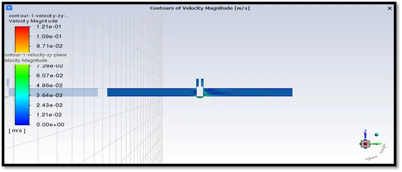
Fig: Velocity contour at cut section plane for fluid flow (inlet=left)

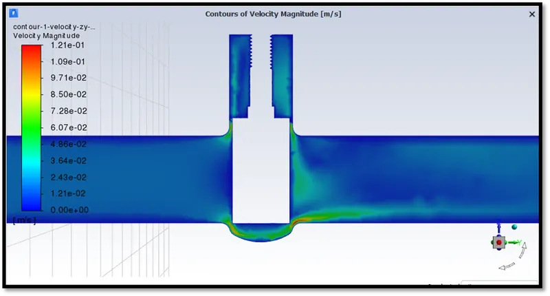
Fig: Close up view of velocity contour at cut section plane for fluid flow (inlet=left)

The flow coefficient and flow factor values are put in the table below.

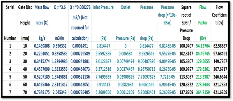
Fig: Flow coefficient and Flow Factor values – Table

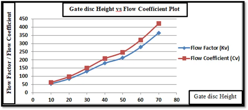
The flow factor and flow coefficient values increase as the gate disc height increases.

CONCLUSION

The gate disc level shows a maximum mass flow rate as the level is increased. This causes more fluid flow. At the gate disc section, the velocity will be very high for increased pressure at the inlet to accommodate the conservation of mass and momentum as fluid progresses towards outlet following the Bernoulli’s principle. The gate valve plays an important role in maintaining the fluid flow rate which increases with increase in the gate disc levels against acting as a barrier to fluid flow. The flow coefficient value increases by 56.07%. The difference percentage for flow coefficient between 10mm height and 20mm height of gate disc opening is 43.79%. The flow coefficient increases by 31.03% for cases 6 and 7 consisting of 60mm and 70mm gate disc height. The gate is usually fully opened or closed. Partial opening of the gate disc causes vibrations which impact and induce damage to the gate valve.

References

[1]

https://www.academia.edu/32423551/A_Review_on_Design_and_Analysis_of_Gate_valve_using_Various_Computer_Aided_Techniques

[2]

https://www.researchgate.net/publication/315747877_DESIGN_AND_ANALYSIS_OF_GATE_VALVE_BODY_AND_SEAT_RING_Design_and_Analysis_of_Gate_Valve_Body_and_Seat_Ring