Week 8 - Simulating Cyclone separator with Discrete Phase Modelling

Introduction to GUI based CFD using ANSYS Fluent

Cyclone Separator – DPM - Report

B A Mayur

INTRODUCTION

A cyclone separator is a device built to remove particulate matter whose size varies in a certain range above or below which they cannot be controlled or are effective. A cyclone separator is an economical device for removing particulate solids from a fluid system. The sizes usually are larger than 10micrometers in diameter. Inexpensive and efficient cyclone separators are available that remove particulate matter as small as 2.5 micrometers. They are not very effective when large particulate matter (200 micrometer) come into play. Devices such as gravity settling chamber or momentum separators are a better option for removal of large particulate matter. Cyclone separators are used in industrial applications such as power generations, gas turbines and chemical processes.

Keywords: DPM, tracking parameters,

AIM

• To calculate the efficiency of the cyclone separator by varying velocities and particulate diameter using discrete phase modeling
• To obtain the pressure drop for all cases and visualize the vortex contours by exporting the particle tracking data into CFD Post.

THEORY OF THE PROBLEM

Cyclone separators are made such that their design of the inlet and two outlets are positioned in such a way that particulate matter is removed using a swirl motion within the separator. This swirl motion and the tapered geometry towards outlet enhance the separation of the discrete phase (particulate matter) from the continuous phase (fluid). Particle tracking option helps to retrieve information on the amount of particulate matter that has been let out from the chamber. They follow a swirl like motion which helps in separation of particles away from the fluid. The induced centrifugal force is tangentially imparted on the wall of the cyclone cylinder. This force, with the density difference between the fluid and solid, increase the relative settling velocity. The settling velocity also referred to as sedimentary velocity is defined as the terminal velocity of a particle in still fluid. A particle in stationary air will settle under the action of gravity and reach a terminal velocity quite rapidly.

Four empirical models used to calculate the cyclone efficiency are:

1. Iozia and Leith Model :

Iozia and Leith logistic model is a modified version of Barth Model, which is developed based on force balance. The model assumes that a particle carried by the vortex endures the influence of two forces: a centrifugal force, Z and a flow resistance, W.

2. Li and Wang Model :

The Li and Wang model includes particle bounce or re-entrainment and turbulent diffusion at the cyclone wall. A two dimensional analytical expression of particle distribution in the cyclone is obtained. Li and Wang model was developed based on the following assumptions:

• The radial particle velocity and the radial concentration profile are not constant for uncollected particles within the cyclone.
• The tangential velocity is related to the radius of cyclone by: uRⁿ = constant.

3. Koch and Licht Model

Koch and Licht collection theory recognized the inherently turbulent nature of cyclones and the distribution of gas residence times within the cyclone. Koch and Licht described particle motion in the entry and collection regions with the additional following assumptions:

• The tangential velocity of a particle is equal to the tangential velocity of the gas flow, i.e. there is no slip in the tangential direction between the particle and the gas.
• The tangential velocity is related to the radius of cyclone by: uRⁿ = constant.

4. Lapple Model

Lapple model was developed based on force balance without considering the flow resistance. Lapple assumed that a particle entering the cyclone is evenly distributed across the inlet opening. The particle that travels from inlet half width to the wall in the cyclone is collected with 50% efficiency.

GOVERNING EQUATIONS AND OTHER SUPPORTING EQUATIONS

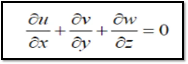
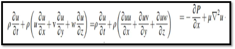
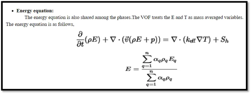
The conservation of mass, momentum and energy equations are used to calculate the problem and validate the analysis.

Conservation of mass equation:

Conservation of momentum equation:

Conservation of energy equation:

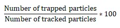
Efficiency (percentage) formula of the cyclone separator:

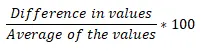
The formula for difference percentage is:

Bernoulli’s Principle Formula:

The Bernoulli equation is considered the statement of the energy conservation for the fluids that flow. This is considered to be the qualitative behaviour that lowers the pressure in the regions with high velocities. This is termed as the Bernoulli effect.

Problem statement: A 3D simulation is performed to understand the working of a cyclone separator within which a discrete phase is separated from a continuous phase. The clean air is supposed to get out at outlet 1 (upwards, away from gravity). The dirt or particulate matter from the fluid (air) is let out at outlet 2 under the action of gravity and swirl motion where settling velocity helps in the separation of the two phases. According to Stoke’s Law for settling velocity, when the density of the particle is greater than the fluid density, it falls. The particles present in the fluid accelerate until the friction equals the net force of gravity.

SOLVING AND MODELING APPROACH

The simulation is performed using Discrete Phase Modeling (DPM). DPM is employed to represent solid particles in gas or liquid or liquid droplets in gas (Ex: Bubbles in liquid). The discrete phase modeling approach considers two phases.

1. Continuous phase

It consists of the fluid flowing within the fluid volume

1. Discontinuous phase

It consists of the smaller particles that are supposed to be interacting with the continuous phase.

The discrete phase can exchange momentum, mass and energy with the fluid phase (i.e., the continuous phase).

The geometry is imported as a .stp file into SolidWorks for a view of dimensions.

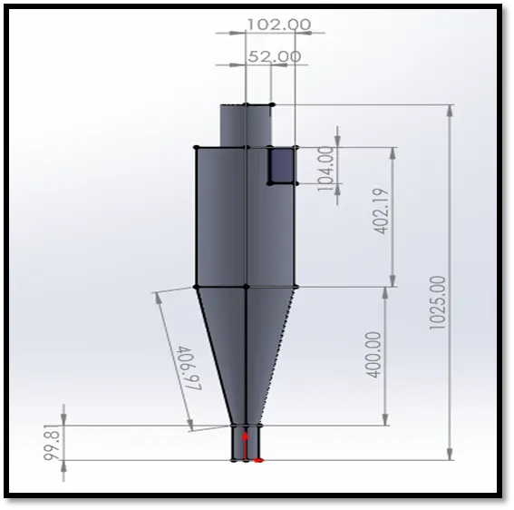
Fig: Front Plane Dimensions

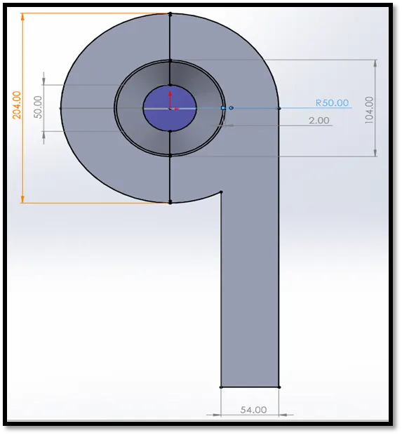
Fig: Top Plane Dimensions

The ‘named selections’ for surfaces is created for setting up the boundary conditions of inlet, wall and two outlets of the cyclone separator.

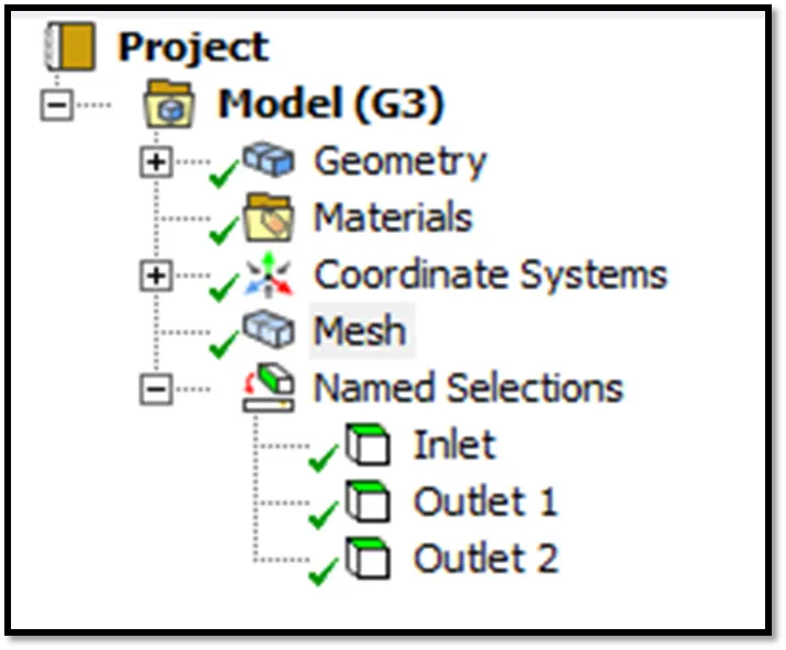
Fig: Named Selections

The mesh is conducted with an element size of 5.35mm and 10mm for all cases. Below is an image of mesh statistics

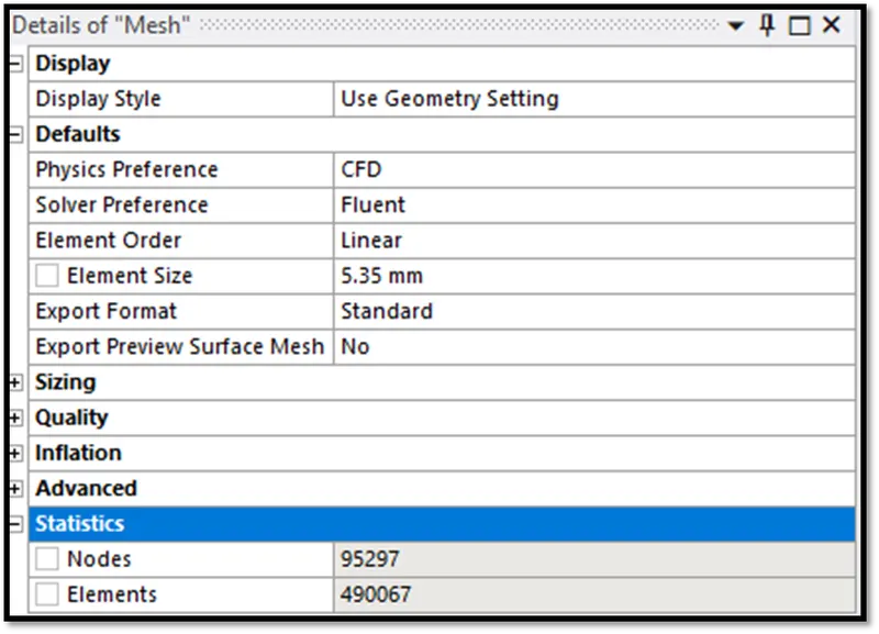
Fig: Mesh statistics

An image of the model after meshing is shown below.

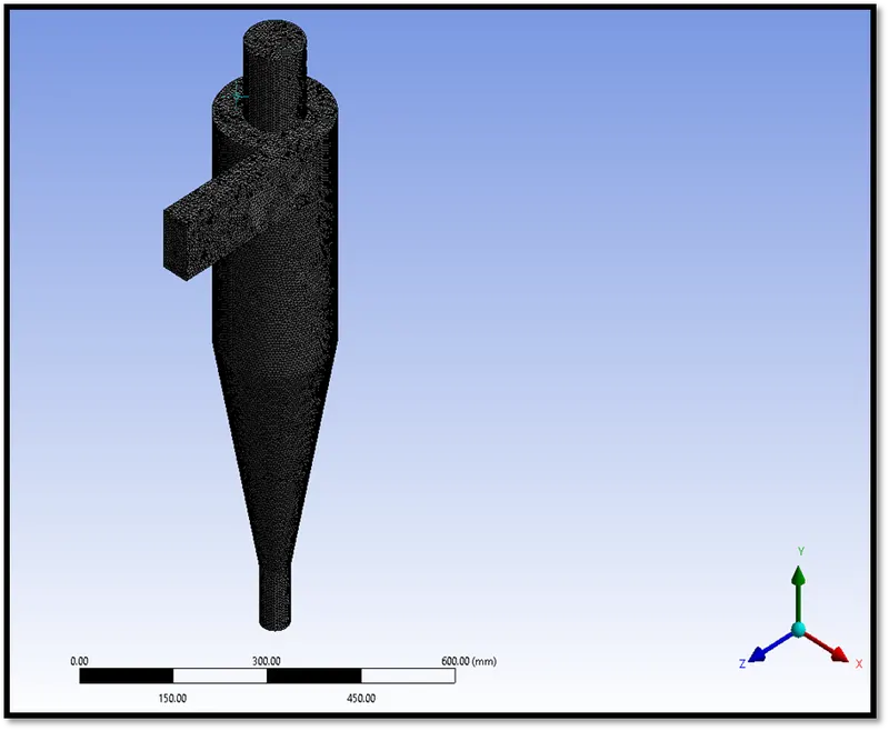
Fig: Mesh model for simulation

Mesh Details Table
Case	Overall Mesh Element Size (mm)	Cells	Faces	Nodes
Case ‘i’ –	5.35	490067	1006629	95297
Case ‘ii’ –	10	111627	231272	22771

A structured Cartesian quad mesh gives better results as the cell centers will be aligned, however the tetrahedral mesh has been used to produce the computational mesh in this report.

TURBULENCE MODELS

The turbulence model helps to specify the correct model needed for the simulation. An RNG k-e turbulence model is used to perform the simulation as this model can consider the swirl motion. RNG k-e model is a slight modification of the standard k-e model which enhances the accuracy of swirling flows. RNG options enable swirl dominated flows.

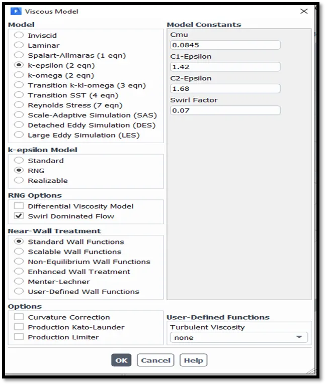
Fig: RNG k-e turbulence model with swirl dominated flow option enabled

PRE-PROCESSING AND SOLVER SETTINGS

A pressure based solver with a steady state approach is used for the simulation.

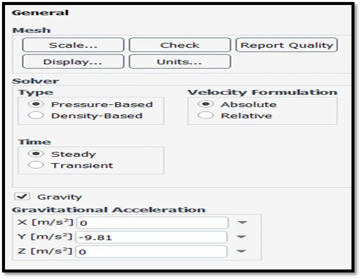
Fig: General conditions

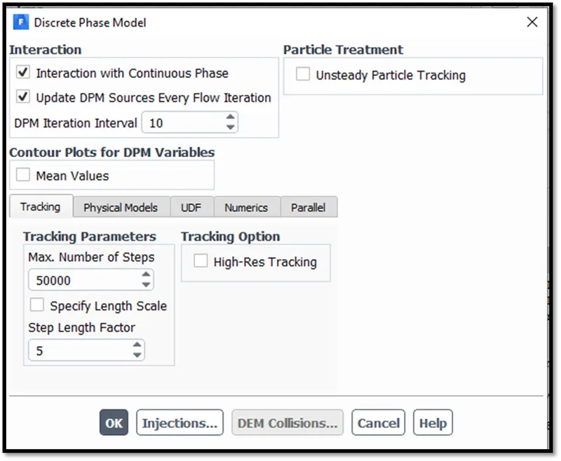
Fig: Discrete phase modeling settings – Case (i)

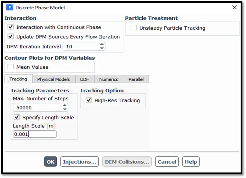
Fig: Discrete phase modeling settings – Case (ii)

The discrete phase modeling settings have ‘interaction with continuous phase’ and ‘update DPM sources every flow iteration’ options turned ON. They enable the solid particles of the discrete phase to have a coupled interaction with the fluid or the continuous phase. This is called as coupled flow where the discrete phase (anthracite) will influence the flow of the continuous phase. Since the size of the particles injected into the cyclone separator is very small (1e-6m), the usage of any type of flow will usually not matter much. The ‘update DPM sources every flow iteration’ option calculates particle source terms at every iteration. This option is very well recommended for un-steady flow simulations; however we use the option in this case as well. The DPM iteration interval option allows the user to control the frequency at which the particles are tracked. If we specify a higher interval, it will technically be computationally less heavy.

Tracking parameters: It is the maximum number of time steps to compute a single particle’s trajectory. In case Fluent exceeds these number of time steps, it will automatically cancel the reporting of the trajectory.

If a certain particle is trapped within a re-circulation region, by specifying the maximum number of steps, we can stop Fluent from tracking that particular particle infinitely. 50000 time steps for steady state simulation is default. We can increase this number to evaluate the trajectory if the user is sure that the particle will be getting out of the recirculation zone.

Smaller value of length scale increases the accuracy of the trajectory by providing small time step size. The larger the step length factor is, the smaller the time step will be. The discrete phase model settings have been changed to a length scale of 0.001m for case ‘ii’, 10 mm element mesh size.

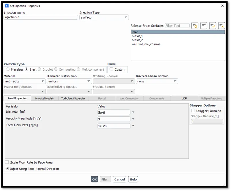
Fig: Injection settings at inlet

The injection type is mentioned as ‘surface’ at inlet along with a particle flow rate (1e-20kg/s) as shown in the image. The particle type is inert (not mass-less type), material is set to anthracite with a certain velocity in the ‘set injections properties’. These are the injection settings to inject the particles with the fluid phase whose velocity is also mentioned as 3m/s at inlet.

Other boundary condition setting for the inlets, outlets and walls are shown below.

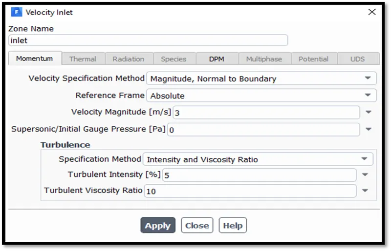
Fig: Inlet velocity = 3m/s

The velocity for the continuous phase or the flow velocity is mentioned as 3m/s for Case ‘A’. The particle diameters are varied for cases ‘B’ and ‘C’.

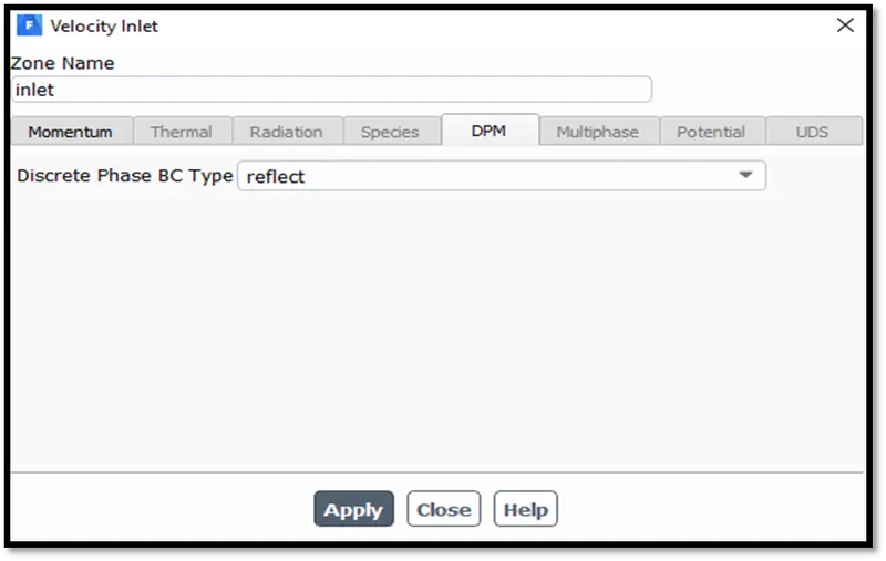
Fig: Inlet Discrete Phase BC type is reflect

The inlet discrete phase boundary condition type is set to reflect. This boundary conditions type does not entertain the capture or trapping of the particles, instead it reflects or sends the particles inward, normal to the surface of the inlet.

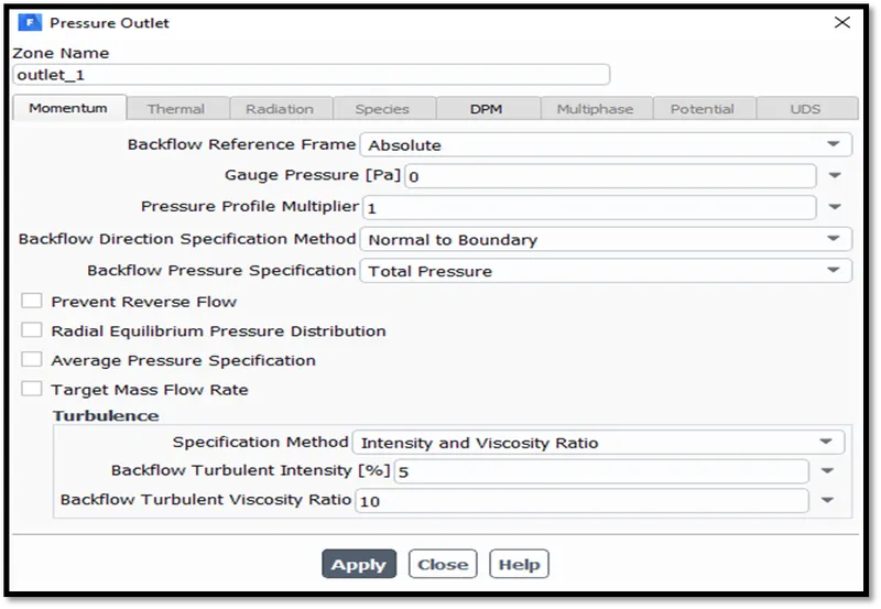
Fig: Outlet 1 (against gravity) boundary conditions

The outlet 1 is the outlet vent opposite to outlet 2 where the clean air is let out. The boundary conditions are mentioned as shown in the images.

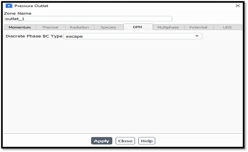
Fig: Outlet 1 Discrete phase BC type is escape

The outlet 2 discrete phase boundary condition type is set to escape. Here the particles can escape from the outlet section which is counted for calculation of efficiency. The ‘escape’ option does not let the particulate matter to flow out of the outlet 1. It allows the clean air only to be separated.

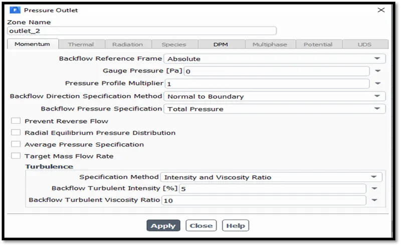
Fig: Outlet 2 momentum boundary conditions

The outlet 2 facing the gravity component is where the particles are trapped or counted for calculating the efficiency of the cyclone separator. Hence the discrete phase boundary condition type is set to escape as well where particles can be let out of the outlet surface.

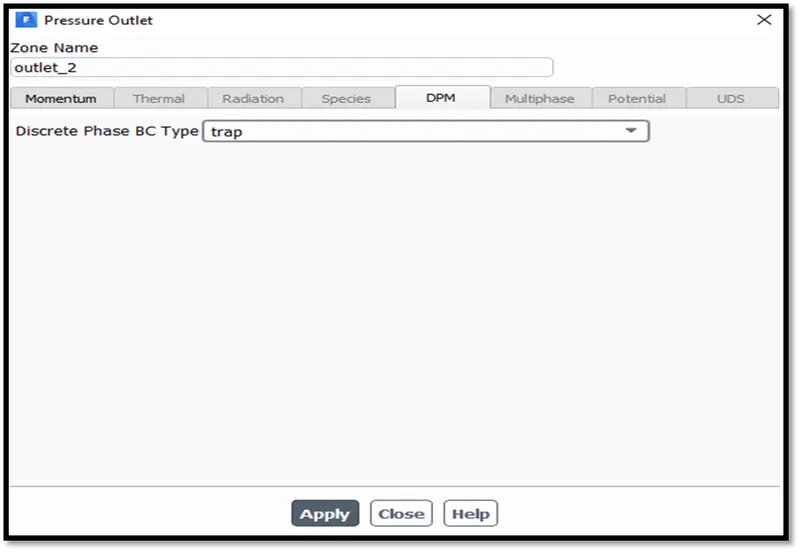
Fig: Outlet 2 Discrete Phase BC is set to trap

The “Prevent Reverse Flow” option has been enabled for Case ‘ii’ for Outlet 2 (bottom).

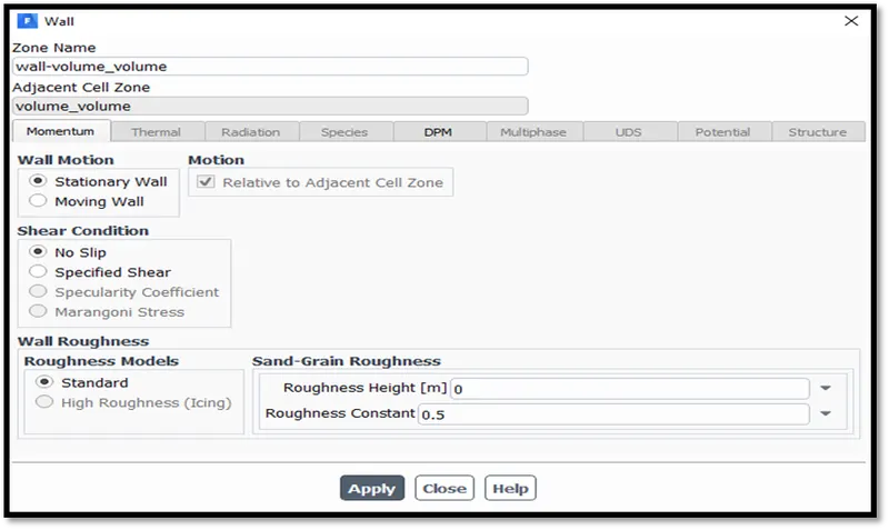
Fig: Wall momentum boundary conditions

The walls of the cyclone separator are the surfaces which enclose the swirling within the separator and houses the inlet and two outlets considering the tapered geometry. They have the ‘no-slip’ condition specified which means that frictional forces are considered during the calculation.

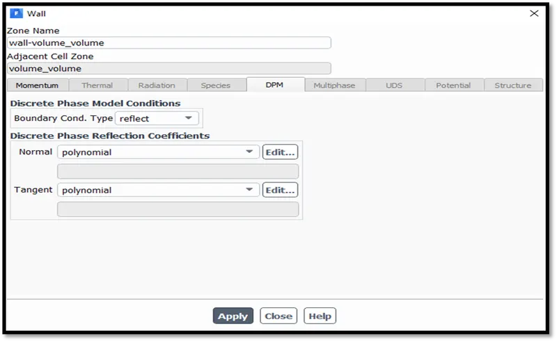
Fig: Wall DPM BC type is set to reflect

The wall discrete phase boundary condition is set to reflect as well. They help the particles to bounce back in the solution domain to be separated under the swirl action within the geometry.

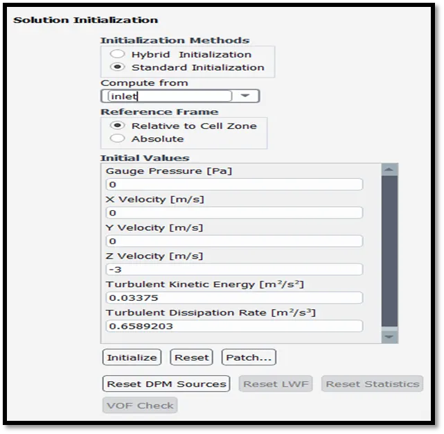
Fig: Solution is initialized (Standard)

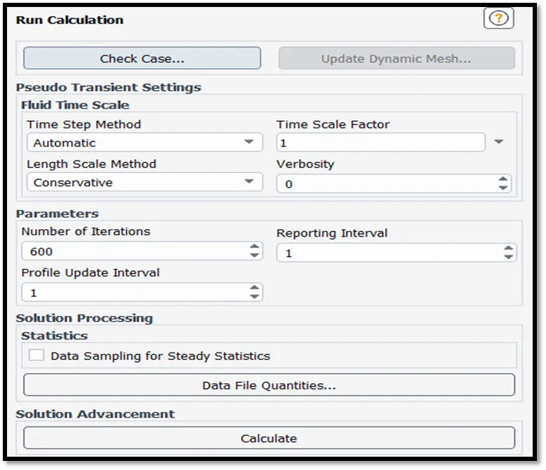
Fig: Calculation settings

The time scale factor is specified as 1 and calculation is run for 600 iterations for all cases.

The scaled residuals plot image is shown below. The solution was converged around 266^th iteration.

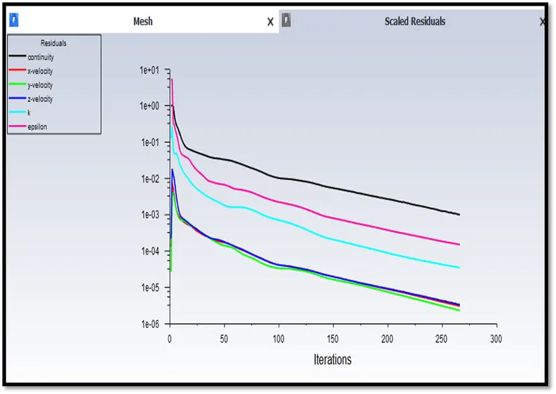
Fig: Scaled residuals for case ’A’

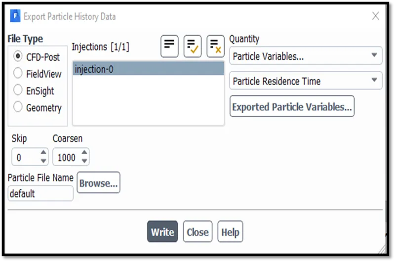
Fig: Particle History Data Export

The particle tracking data is then imported into CFD post for viewing information of the vortex zones, particle path (trajectory tracking) and trapped particles information.

RESULTS

(i) Element size of 5.35mm

The cases ‘A’, ‘B’ and ‘C’ have velocities set to 3m/s. The cases ‘D’, ‘E’ and ‘F’ have particulate matter diameters of discrete phase flow set to 5𝝁m (5 x 10^-6 m).

Case i	Tracked	Escaped (Outlet1)	Trapped (Outlet 2)	Incomplete	Efficiency (in %)
Case ‘A’ – 1𝝁m	368	78	20	270	5.434
Case ‘B’ – 3𝝁m	368	45	108	215	29.34
Case ‘C’ – 5𝝁m	368	-	156	212	42.39
Case ‘D’ – 1m/s	368	48	16	304	4.34
Case ‘E’ – 3m/s	368	-	156	212	42.39
Case ‘F’ – 5m/s	368	-	367	1	99.72

(ii) 10 mm mesh element size

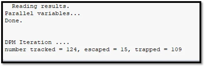
Fig: DPM values for case (ii) ’A’

Case ii	Tracked	Escaped (Outlet1)	Trapped (Outlet 2)	Incomplete	Efficiency (in %)
Case ‘A’ – 1𝝁m	124	15	109	-	87.90
Case ‘B’ – 3𝝁m	124	17	107	-	86.29
Case ‘C’ – 5𝝁m	124	-	116	8	93.54
Case ‘D’ – 1m/s	124	9	115	-	92.741
Case ‘E’ – 3m/s	124	1	114	9	91.93
Case ‘F’ – 5m/s	124	-	124	-	100

The pressure drop for all cases was recorded between inlet and outlets in Pascals.

Case ‘ii’	Pressure Drop at Outlet 1 (Pa)	Pressure Drop at Outlet 2 (Pa)
Case ‘A’	7.2311218	13.359141
Case ‘B’	7.2653451	13.422936
Case ‘C’	7.0704675	13.061527
Case ‘D’	0.67944082	1.2550663
Case ‘E’	7.0704675	13.061527
Case ‘F’	20.415935	37.717217

The results for case ’i’ comprising of 5.35mm mesh element size have been performed with different tracking parameters under discrete mesh model settings. Hence the results have a huge deviation. They could be corrected but the cost of computation would be rather high. Hence the simulations were performed for 10mm mesh element size with length scale of 0.001m at high resolution tracking. The results are satisfactory for the required objective.

Under case ‘ii’, we can see that the cases ‘A’, ‘B’ and ‘C’ have similar pressure values as the velocity is kept constant. For cases ‘D’,’E’ and ‘F’ the pressure drop values are changing as the velocity increases with constant particulate matter diameters of 5e-6m.

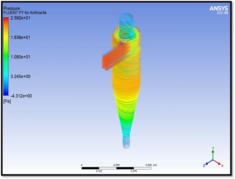
Fig: Pressure distribution contour – Case ‘A’ – CFD Post

The file has been save using the ‘export – write’ option from fluent and imported into CFD Post for visualization of contours and particle tracking information.

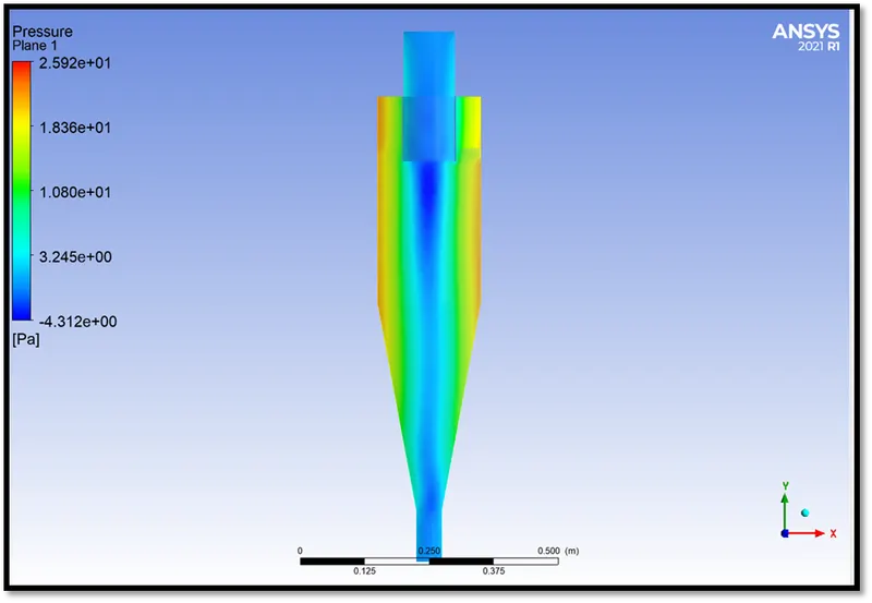
Fig: Pressure contour 2D at mid-plane – Case ‘A’ – CFD Post

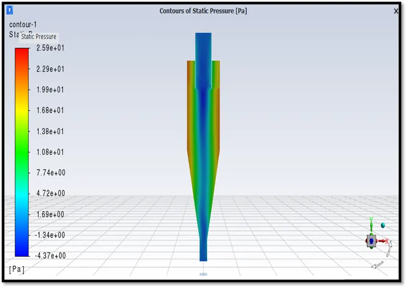
Fig: Pressure contour 2D at mid-plane – Case ‘A’

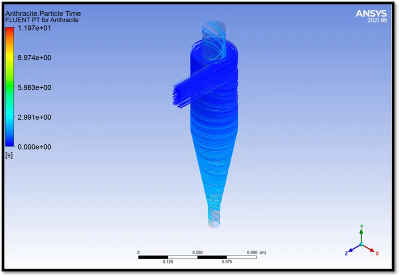
Fig: Anthracite Particle Time

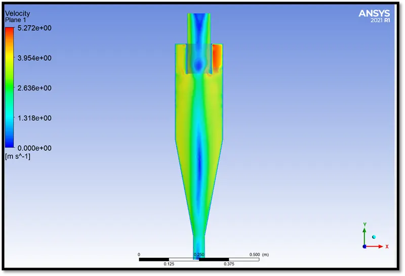
Fig: Velocity contour 2D – Case ‘A’ - CFD Post

There is a high velocity near inlet. The velocity decreases due to the swirling flow effect, acceleration due to gravity and friction near walls of the fluid domain.

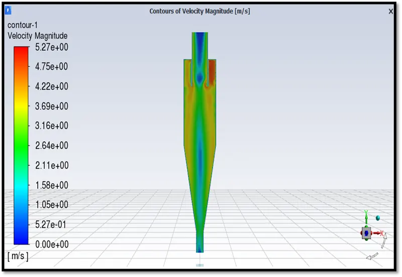
Fig: Velocity contour 2D – Case ‘A’ at distance 0.01m – XY Plane

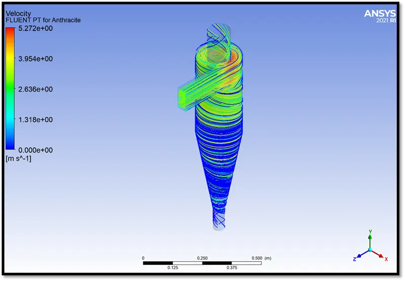
Fig: Velocity Streamlines contour 2D – Case ‘A’ - CFD Post

Micro-inter circulation zones called vortex zones will be created within the geometry of the model. The vortex zones are shown in the image below.

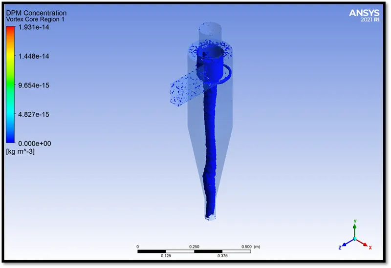
Fig: Vortex zones at 0.05 level of swirling strength (Value = 39.32s^-1) – Case ‘A’

Because of the vortices and the influence of the swirling flow, the clean air moves upward after overcoming the division immediately after the inlet pass (i.e., fluid goes down to overcome the geometry stopping it from entering outlet 1 directly and then clean air is pushed upward in Y direction). The fluid flows where the pressure difference is negative i.e., at outlet 1 (air flows from higher pressure to lower pressure). The swirling strength goes up to 786.584 s^-1. It is the maximum value of the vortex swirl range which was measured in CFD Post. The swirl strength only signifies that as the radius is low, towards the center of the swirl, the swirl strength is higher. It is an inverse of time (frequency, s^-1).

CONCLUSION

The results for case ‘ii’ have a closer tendency to provide satisfactory results due to the tracking parameters and also considering the computational cost. The cases ‘B’ and ‘C’ have the highest difference in pressure drop at outlet 2 of 2.729% for constant velocities of 3m/s.

The difference percentage for case (ii) ‘F’ (5m/s) between pressure drops at outlet 1 and outlet 2 is 59.522%. The difference percentage for case (ii) ‘D’ (1m/s) between pressure drops at outlet 1 and outlet 2 is 59.51133%.

However, for constant velocities, the case (ii) ‘B’ has shown a pressure drop difference between inlet-outlet_1 and inlet-outlet_2 of 59.5733%, similar to values shown by cases ‘A’ and ‘B’.

References

[1]

https://www.ijser.org/researchpaper/DESIGN-AND-ANALYSIS-OF-CYCLONE-SEPARATOR.pdf

[2]

https://www.researchgate.net/publication/312160127_Design_and_fabrication_of_cyclone_separator

[3]

https://www.sciencedirect.com/science/article/pii/S0307904X06000291

https://doi.org/10.1016/j.apm.2006.03.011

[4]

https://www.researchgate.net/publication/232747389_A_CFD_Study_on_the_Prediction_of_Cyclone_Collection_Efficiency

DOI:10.1080/15502280590923649

[5]

http://dspace.unimap.edu.my/xmlui/bitstream/handle/123456789/13571/054-058_empirical%20models.pdf?sequence=1#:~:text=This%20study%20reviews%20the%20prediction,Iozia%20and%20Leith%20%5B4%5D.