Week 5 - Rayleigh Taylor Instability
Introduction to GUI based CFD using ANSYS Fluent
Mixing Tee Report
B A Mayur
Introduction
For free surface boundaries, the volume of fluid method is used to understand the interaction between two fluids of different phases. It is an important method to simulate 2 phase flows. In this 2D analysis, the VOF method provides information of the interaction between the two fluids by visualizing the boundaries of the fluids. Rayleigh Taylor Instability is the inter-penetration at the interface shared between two fluids of varying densities. The interface becomes unstable as the heavier fluid penetrates into the lighter fluid.
AIM
- To perform a multiphase simulation of Rayleigh taylor Instability
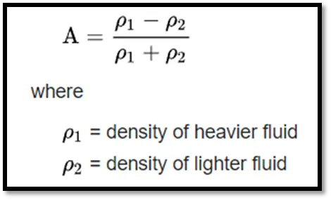
- Calculation of Atwood Number
THEORY OF THE PROBLEM
The instability problem considers air and water and tracks volume mixing between the two surfaces. Air and water fluid material parameters are set using the Fluent database and simulation is performed for the two phases using the Multiphase option in ANSYS Fluent 2021 R1. The interaction of the two fluids is depicted as both have different densities and mixing effects are captured. This happens due to the two phases being different in nature. A dense fluid is modeled on top and air (lower density) is modeled below water and simulation performed. The instability predicted is enhanced due to gravity effects at their interface. The Rayleigh Taylor is used in simple distillation processes. The interface between the two fluids becomes unstable with respect to time as densities vary and pressure waves are created causing a force imbalance between the two. This breaks the interface and enhances inter-penetration.
The volume of fluid method is economical to track free boundaries in 2D or 3D grids. It is also more efficient and flexible than the finite difference method.
The Eulerian approach focuses on changes occurred at a fixed point with respect to time and space (particles interacting/moving at this point). The Lagrangian approach tracks and predicts a fixed particle in time and space in a control volume.
GOVERNING EQUATIONS AND OTHER SUPPORTING EQUATIONS
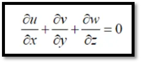
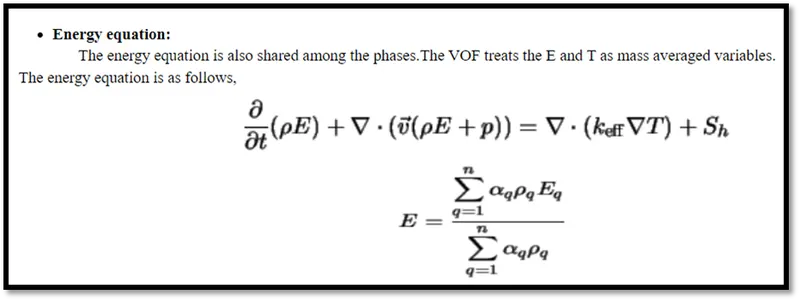
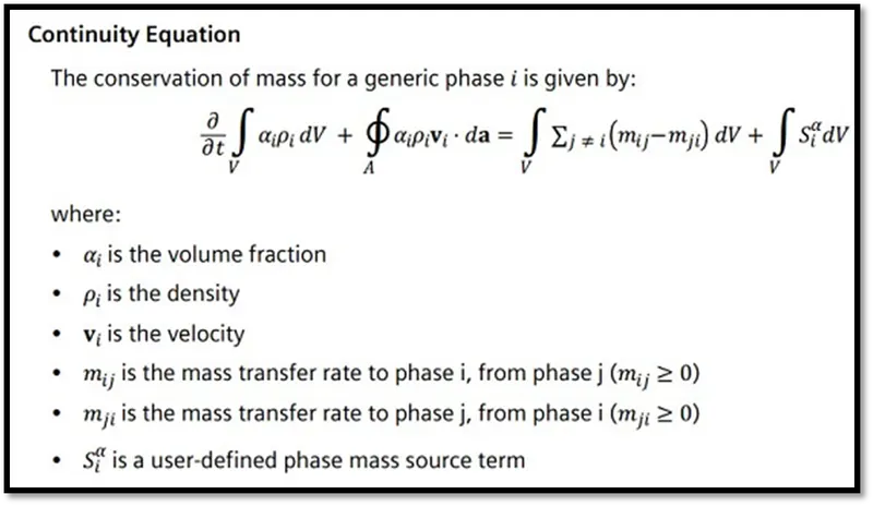
The conservation of continuity, momentum and energy equations is used to calculate the problem and validate the analysis.
Conservation of mass equation:
Conservation of momentum equation:

Conservation of energy equation:
The formula for difference percentage is:
Atwood number (A): Dimensionless density ratio used to study hydrodynamic instabilities in density stratified flows.
Volume of fluid equations; Volume fraction equation:
SOLVING AND MODELING APPROACH
The water and air domains are created as phases in the 2D mesh generated. Firstly, a square of 20x20 mm is created for air. Similarly another surface is created for water above the air domain.
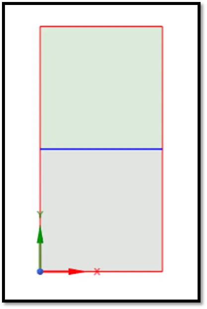
Fig: Water and air domains created using Pull tool in SpaceClaim
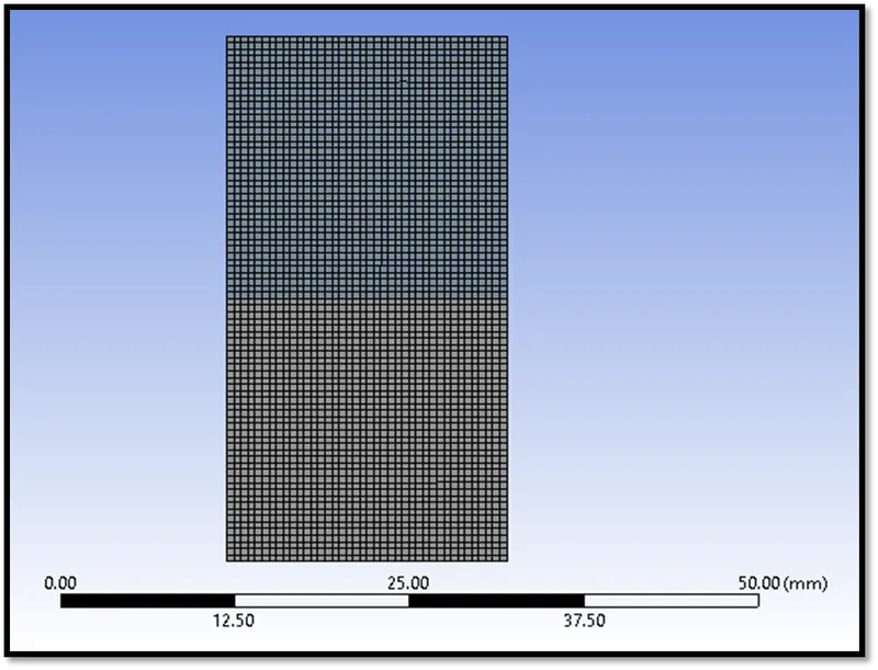
Fig: Mesh display of the 2D domain for water (above) and air
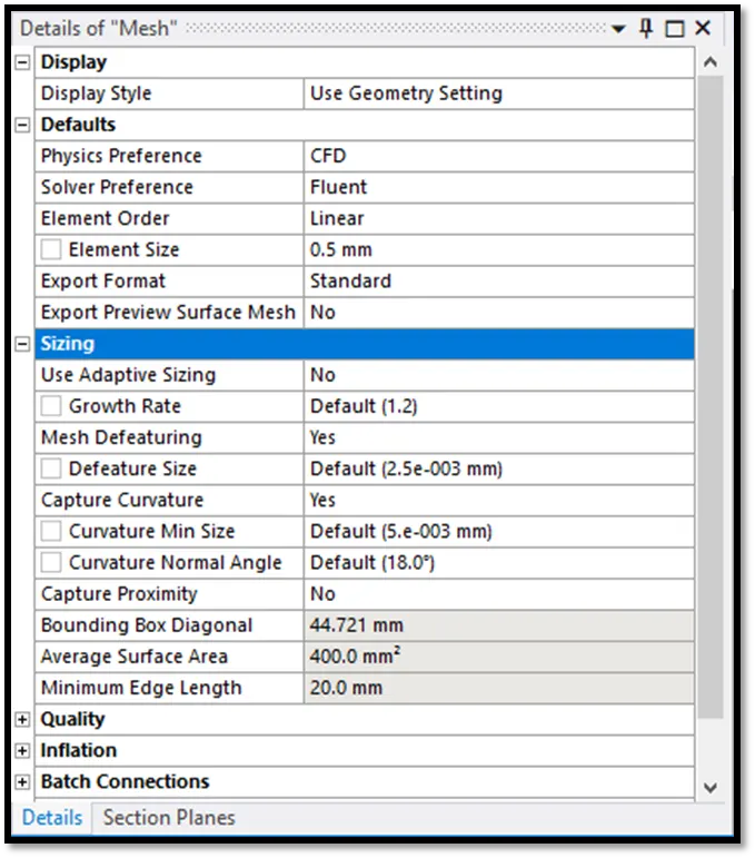
Fig: Mesh Details
For a conformal mesh, “SharePrep” tool is used to make a shared edge between the two domains and interface created.
TURBULENCE MODELS
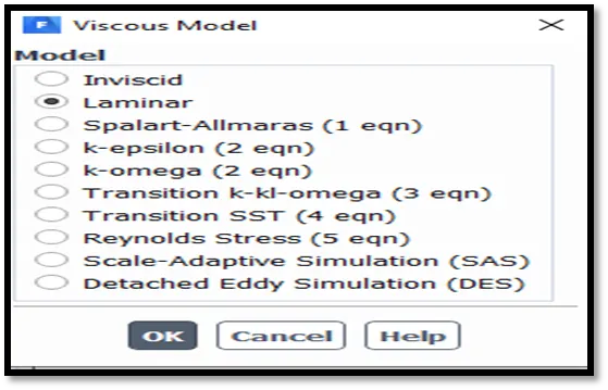
The model specifies options for control of the flow. Here the laminar flow option is selected which specifies that the flow is not turbulent in nature and the flow has a low Reynolds number.
PRE-PROCESSING AND SOLVER SETTINGS
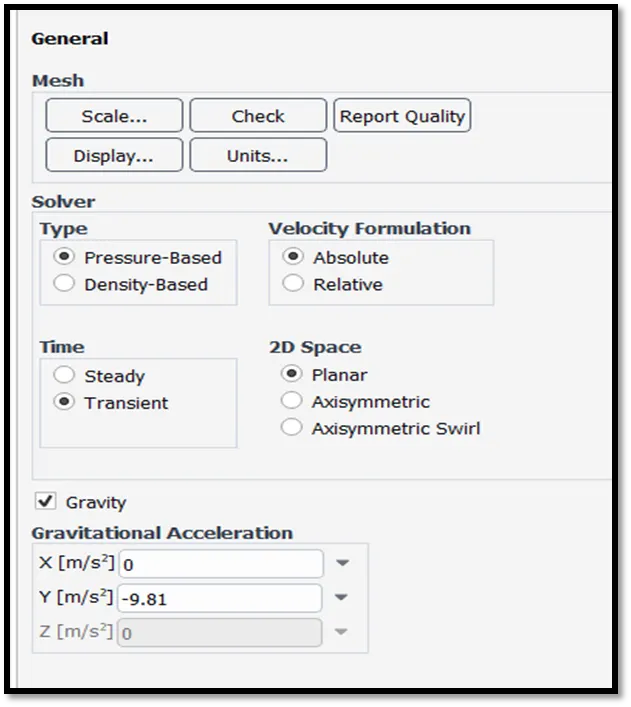
There is no need of turning on the energy equation as thermal parameters are not of considered. The data is taken from Fluent database as default settings for air and water. We enable gravity to -9.81m/s for y axis as this stimulates in the interaction/mixing effect.
The multiphase model using Volume of Fluid method is chosen for the two Eulerian phases (air and water).
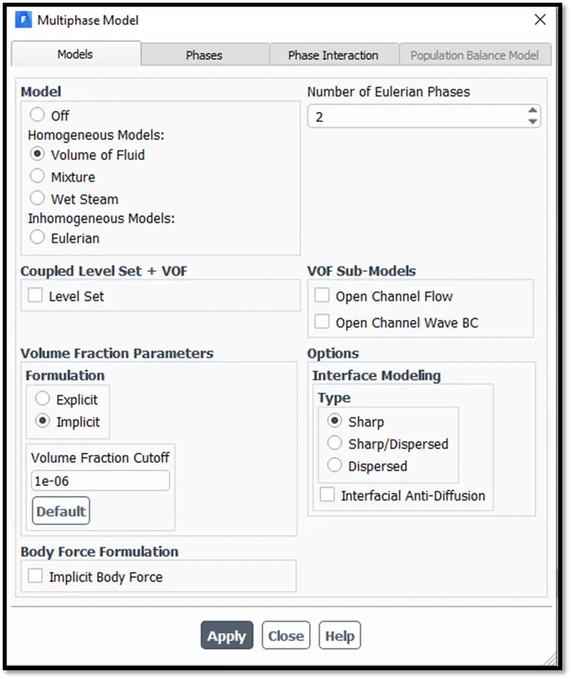
The courant number is an explicit criteria to ensure that the time step value is not very high to capture results. Here, the implicit method is used.
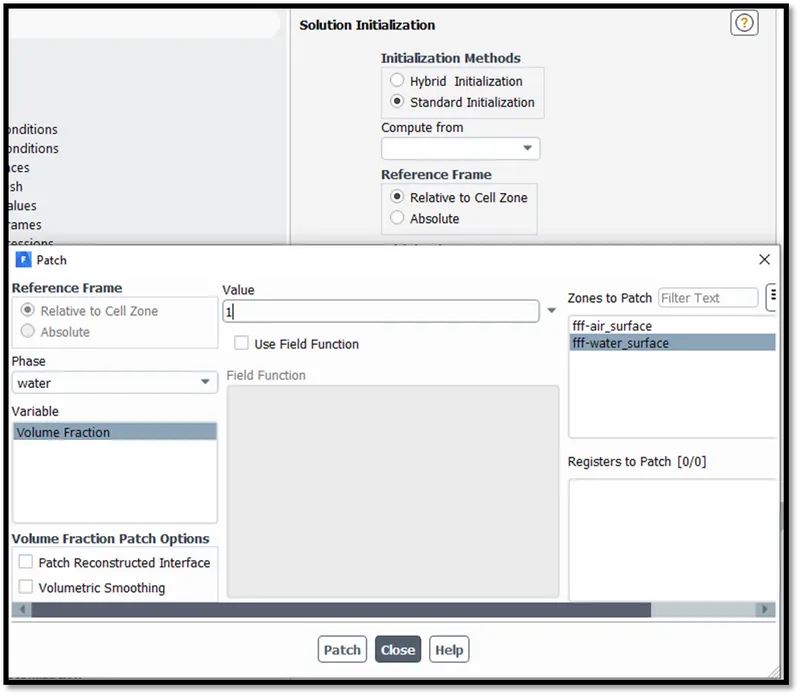
During initialization, the “Patch” option is used to patch the two domains i.e., air and water using the water fraction variable and enabling value to 1 for water.
The number of time steps is set to 1500 with a time step size of 0.01 for the transient approach using a pressure-based solver to see how the interface collapses as a function of time. The maximum iterations per time step are specified as 40.
SIMULATION WITH 3 DIFFERENT MESHES
|
Mesh Element Size (in mm) |
Cells |
Nodes |
Faces |
|
0.5 (base mesh) |
3200 |
3321 |
6520 |
|
0.3 |
8978 |
9180 |
18157 |
|
0.2 |
20000 |
20301 |
40300 |
The interface changes with respect to time as the boundaries fluctuate thereby allowing air to move upwards and water domain pushed downwards due to gravity and density effects. The simulation effects captured also vary with different mesh sizes. The flow visualization predicted turns out to show a smoother transition from two separated domains, mixing and followed by separation again due to gravity as the mesh element size decreases. The ’alpha’ value or the volume fraction is 1 at top for water and 0 at the bottom of the interface for air.
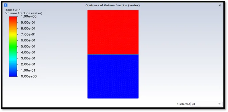
Fig: Phase contour at initial stage for 0.1 mesh element size
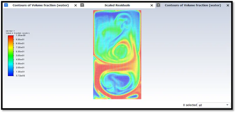
Fig: Simulation flow captured at 2% for 0.3 mesh element size at 1500 time steps, 0.01s per time step and 40 iterations specified
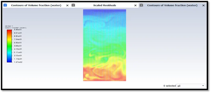
Fig: Simulation flow captured at 9% for 0.3 mesh element size at 1500 time steps, 0.01s per time step and 40 iterations specified
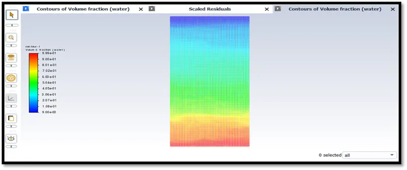
Fig: Simulation flow captured at 16% for 0.3 mesh element size at 1500 time steps, 0.01s per time step and 40 iterations specified
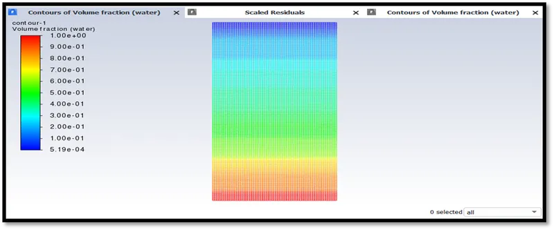
Fig: Simulation flow captured after calculation is completed for 0.3 mesh element size at 1500 time steps, 0.01s per time step and 40 iterations specified
RESULTS
The flow simulation images for different mesh sizes at 10th time step using animation playback option are given as follows.
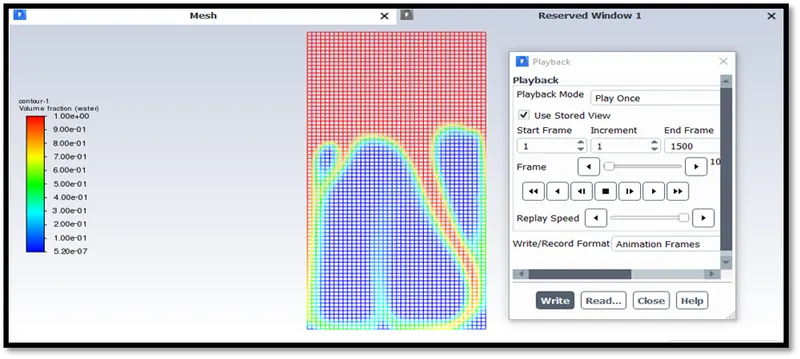
Fig: 0.5 mesh element size
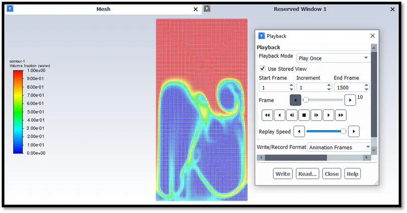
Fig: 0.3 mesh element size
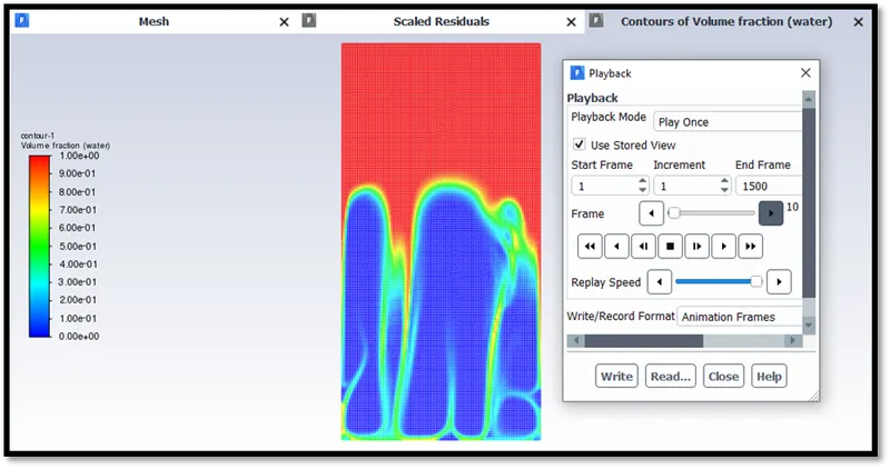
Fig: 0.2 mesh element size
A floating point error during the simulation at 0% was found for the 0.1 mesh element size having 1500 time steps with 40 iterations per time step calculated at 0.01s for the time step size. This is because as numerical calculations progress, the residuals tend to zero and divisions cannot be performed causing a floating point error which is off the machine tolerance. The simulation was completed by increasing the mesh size to 0.2 mesh element size under same solver settings.
The scaled residual plots for the three simulations are given as follows.
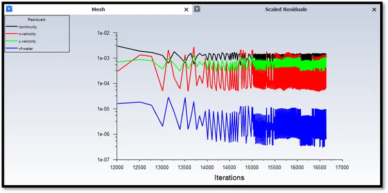
Fig: Residuals plot for 0.5 mesh element size
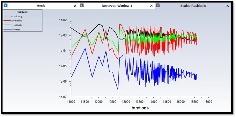
Fig: Residuals plot for 0.3 mesh element size
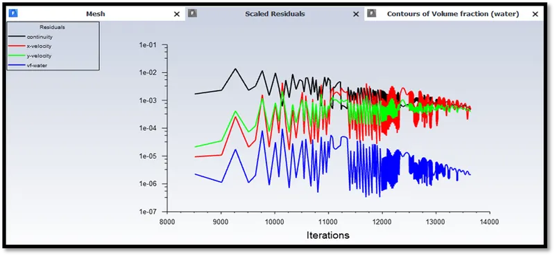
Fig: Residuals plot for 0.2 mesh element size
A simulation was performed using water as the denser fluid and a user-defined fluid having density = 400 kg/m3, viscosity = 0.001 kg/m-s for 0.3 element size refined mesh.
The results are shown below.
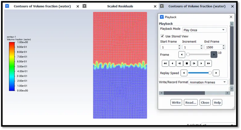
Fig: Simulation at 10th time step for user defined fluid and water
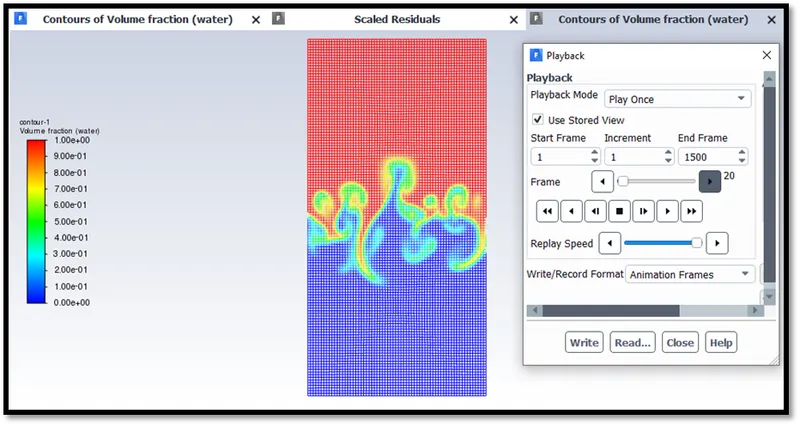
Fig: Simulation at 20th time step for user defined fluid and water
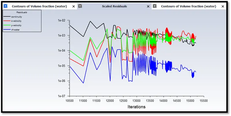
Fig: Residual plot for user defined fluid and water simulation
|
Fluid |
Density |
Atwood Number |
|
Water |
998.2 |
- |
|
Air |
1.22 |
Case 1 (Air and water) – 0.997 |
|
User-defined fluid |
400 |
Case 2 (Water and user defined fluid) – 0.4278 |
CONCLUSION
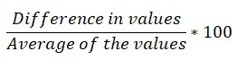
A steady state approach is not suitable for this type of problem as the breaking of the interface is completely time-dependent. We want to simulate the effects and capture the penetration between the two fluids of different densities with respect to time. Hence a transient solver is used to approach the problem. A better flow simulation is captured as mesh is refined following Rayleigh Taylor Instability. The Atwood number difference percentage is 79.89% and the decrease is by 57.091% for simulations performed between water air and user defined fluid as mentioned in the table in the “Results” section.
SIMULATION ANIMATION GOOGLE DRIVE LINKS
- Link for 0.5 mesh element size – air and water multiphase simulation
https://drive.google.com/file/d/143n0TpRABRfWO2SIctv094EetGUMhAgn/view?usp=share_link
- Link for 0.2 mesh element size – air and water multiphase simulation
https://drive.google.com/file/d/143n0TpRABRfWO2SIctv094EetGUMhAgn/view?usp=share_link
- Link for user-defined fluid and water simulation
https://drive.google.com/file/d/1ngMMPZDAiQGAAyRfUHiFJAwFEj62qDR8/view?usp=share_link
REFERENCES
[1] Internet sources
[2] https://www.comsol.com/blogs/modeling-and-simulation-of-multiphase-flow-in-comsol-part-1/