Week 6 - CHT Analysis on a Graphics card
Introduction to GUI based CFD using ANSYS Fluent
Graphics Card Simulation - Report
B A Mayur
INTRODUCTION
A graphics card comprises of a few electronic components, chips (processor) which is mounted on the base, circuits and fins utilized for heat dissipation used in conventional computers. The fins are mounted onto the processor to transfer heat and placed such that the fan/blower is vented directly towards the fins for sufficient heat dissipation. In the simulation the base of the graphics card holds these components. Simulation is performed to understand the temperature distribution and heat dissipation to keep the processor at optimum operation conditions as heat is generated by the processor and transferred to the fins for heat dissipation.
Keywords: CHT (Conjugate Heat Transfer), Heat transfer coefficient
AIM
- To obtain the temperature profiles at different sections of the graphics card
- To understand the CHT approach for different fluid velocities
THEORY OF THE PROBLEM
In this report, the problem statement refers to keeping the processor operations at working temperatures. If the processor heats up over the optimum range, it causes malfunctioning of the processor operations and hence becomes dysfunctional. To avoid the problem, the issue can be solved by mounting a structure having fins through which this heat is conducted. The air blown by a fan onto these fins helps to carry out the heat away from the processor. Using a Conjugate Heat Transfer (CHT) approach, the simulation can be visualized to understand the problem for temperature distribution throughout the model.
GOVERNING EQUATIONS AND OTHER SUPPORTING EQUATIONS
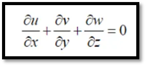
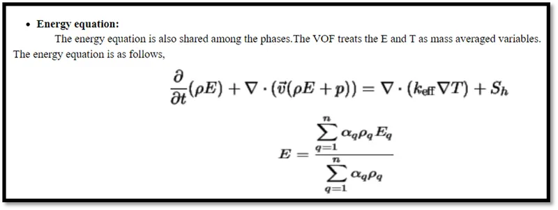
The conservation of mass, momentum and energy equations are used to calculate the problem and validate the analysis.
Conservation of mass equation:
Conservation of momentum equation:

Conservation of energy equation:
Reynolds Number (Re):

Where ‘ρ’ is the density in kg/m3, ‘v’ is the velocity in m/s, ‘D’ is the diameter of the cylinder in meter and ‘μ’ is the dynamic viscosity of the fluid in N/m2.
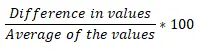
The formula for difference percentage is:
Mass Flow Rate Formula:

Where ‘Q’ is the mass flow rate in kg/m3, ‘A’ is the area of cross section in m2 and ‘V’ refers to the velocity of the fluid. The equation represents the mass flow rates at two varying cross-sections being same for a given fluid.
‘h’ is the Convective heat transfer coefficient, characteristic length in ‘m’ and thermal conductivity of air (W/mk).
Convective Heat Transfer Coefficient:

‘μ’ (in Ns/m2) refers to the dynamic viscosity and Cp is the specific heat capacity in kJ/kg-K. ‘k’ is the thermal heat conductivity in W/mK. Using the equation is sufficient to obtain close results for Nusselt Number, thereby obtaining the HTC value if required for verification.
Problem statement: There are electronic components and fins mated to a rectangular structure. This structure is in turn mounted on the processor and the main base below it. The air is blown with a certain velocity onto the fins and the temperature distribution is visualized, the heat dissipation is checked.
SOLVING AND MODELING APPROACH
The dimensions are shown in images below. The geometry is saved as a .stp 242 file and viewed in SolidWorks software. The simulation is performed for case’A’ – base mesh, case ‘B’ refined mesh and case ‘C’ by mentioning the convective heat transfer coefficient for a conjugate heat transfer (CHT) approach for different inlet velocities.
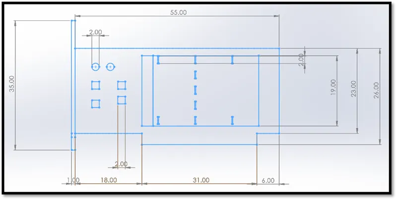
Fig: Dimensions of the simulation model –Front Plane
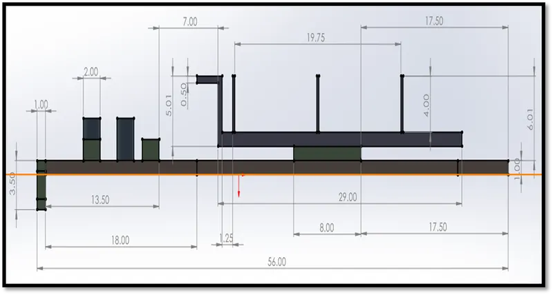
Fig: Dimensions of the simulation model –Top Plane
The dimensions are shown above and simulation is performed on the model. The meshing is performed for a 5mm base mesh and checked against another run with a refined mesh model to obtain accurate results using body sizing method maintaining a conformal mesh. The tetrahedral mesh is set to obtain triangular mesh elements for accurate results. This is also a result of selecting the “shared topology” option in the geometry section. The refined mesh model consists of 0.4 mm element size for the base and fins. The processor has an element mesh size set to 0.3 mm. The length, breadth and height of the processor are 8mm x 8mm x 1mm; (l x b x h).
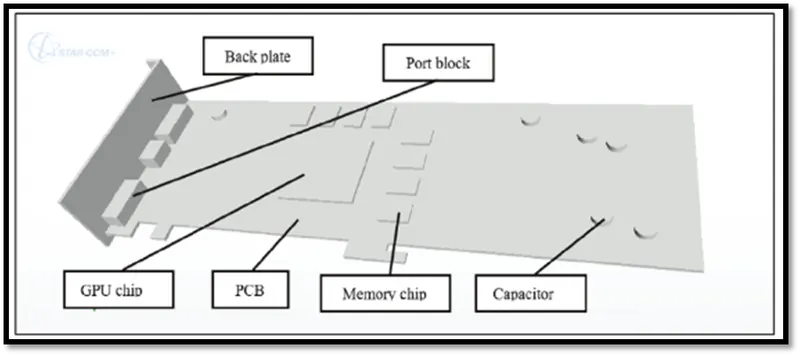
Fig: Internal parts and naming
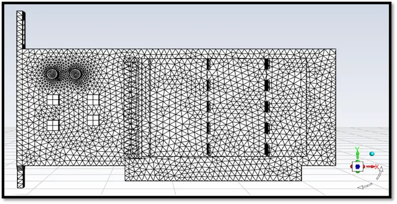
Fig: Graphics Card Mesh Edges - Display perpendicular to XY axis in Setup – base mesh
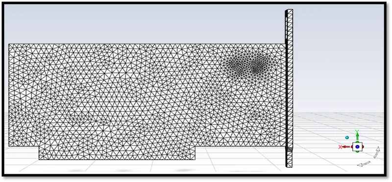
Fig: Graphics Card Mesh Edges - Display perpendicular to XY axis – base mesh (opposite direction)
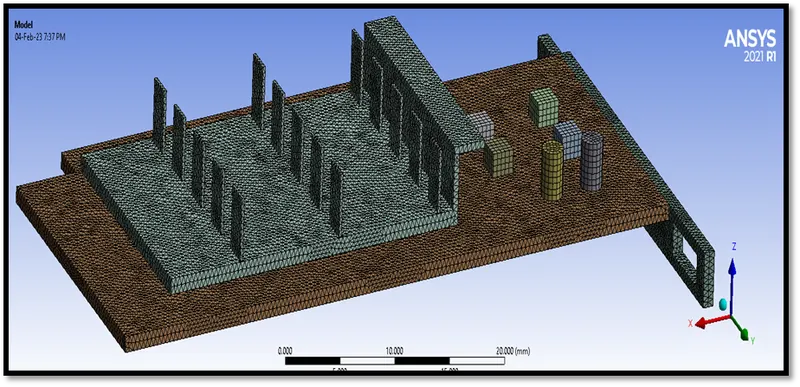
Fig: Mesh display of graphics card (case B) – refined mesh
A base mesh (case ‘A’) is created and then re-defined to a higher degree (case ‘B’ & case ‘C’) to capture the flow effects with the application of body sizing. An SST k-w turbulence viscous model is used to solve the problem with a steady state approach and a pressure based solver as the Mach number is less than 0.3 for the incompressible flow.
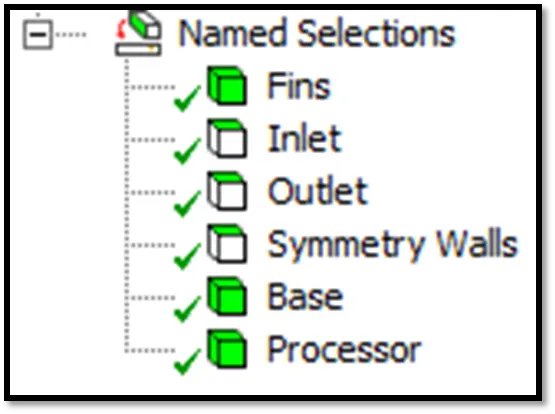
Fig: Named selections
Named selections are made to ensure applying material properties for fins, processor and base. Symmetry walls along with inlet and outlet walls are made to apply boundary conditions and create the enclosure or computational domain for the simulation.
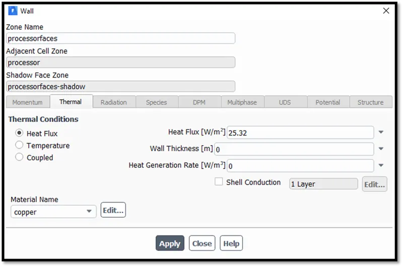
The mesh refinement is performed to obtain a better temperature distribution profile. For case ‘C’, the heat flux value (25.32 W/m2) that has been set will determine the heat transfer rate, also to help produce the post-processing visualizations.
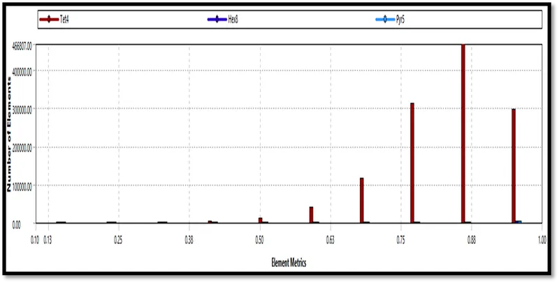
Fig: Mesh metrics
The mesh metrics show a value of 466807 element cells around 80% of tetrahedral cells.
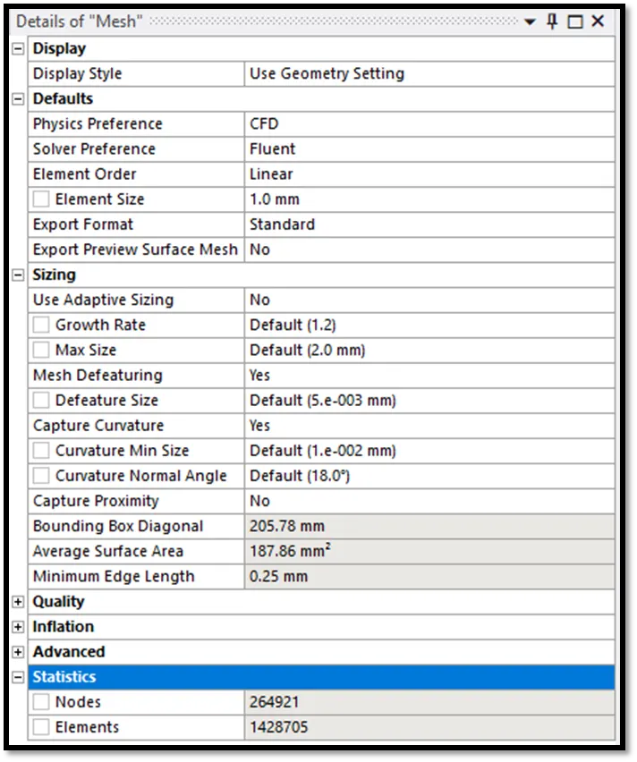
Fig: Mesh display – case ‘A’
The mesh details are shown in the above picture for case ‘A’ and a table follows the mesh details for the different simulations recorded for this report.
|
|
Mesh Details Table |
||||
|
Sl.No. |
|
Overall Mesh Element Size (mm) |
Cells |
Faces |
Nodes |
|
i) |
Case ‘A’ |
1 |
1428705 |
2920300 |
271276 |
|
ii) |
Case ‘B’ |
3 |
1243876 |
2564329 |
248189 |
|
iii) |
Case ‘C’ |
3 |
1243876 |
2564329 |
248189 |
The table above shows the values for number of cells, nodes and faces for the overall mesh element size specified for all cases.
The base of the structure is set to wood, processor as copper and the fins for heat dissipation as aluminum material.
TURBULENCE MODELS
The model specifies options for control of the flow. Here the SST k-w turbulence model works for capturing the results away from the wall as well as near wall using blending functions efficiently. The k-w turbulence model captures the flow effects accurately near wall at adverse pressure gradients and k-e for flow away from walls. Hence a higher y+ value is required for k-e (around 50) and y+ value of 1 or more will be sufficient to capture the results using the k-w turbulence model. The SST k-w turbulence model is a combination of both the turbulence flow models.
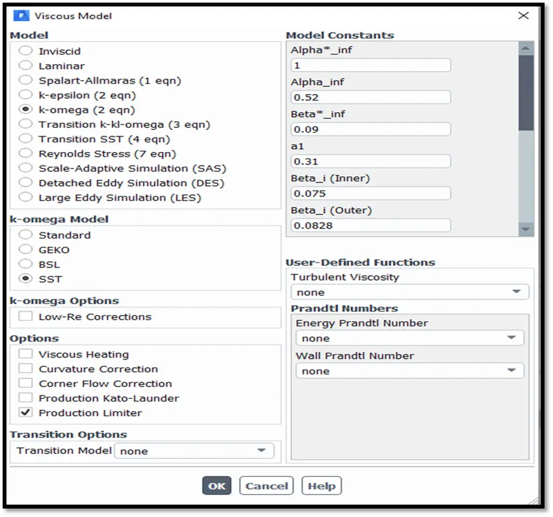
As the velocity is very low, the y+ values for the turbulence models vary between 1-5 and 30-300 for the k-w and k-e models. However models do not have y+ values (inflation layers) specified to perform simulations for this report.
PRE-PROCESSING AND SOLVER SETTINGS
Energy equation is turned ON to set up the thermal parameters and solving conservation of energy equations. This enables to solve for the heat transfer between the solid-fluid blocks.
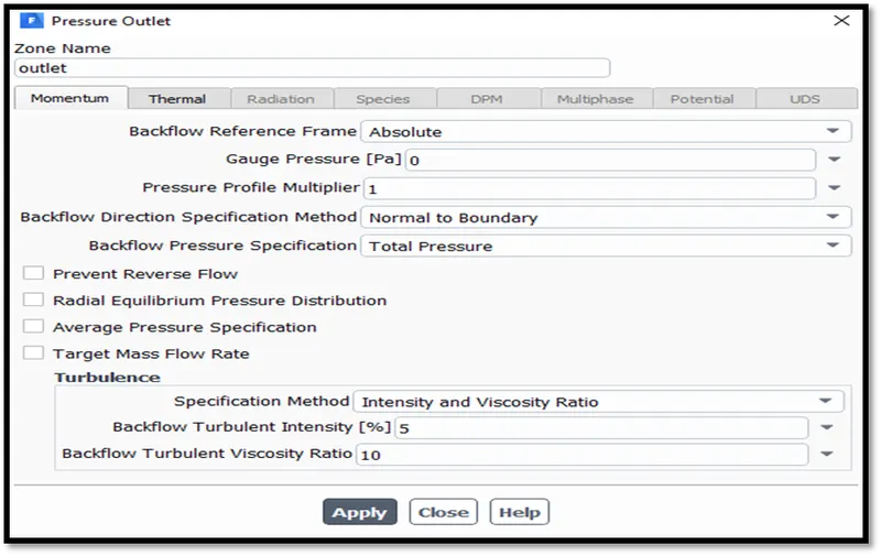
The fluid domain is defined as air and the boundary of the solid-fluid interference is defined as a convective wall. The energy equation is usually turned on to facilitate setting the temperature parameters of the system. The velocity at inlets is set to 1m/s. The gauge pressure is equal to 0 as this is the atmospheric pressure (1atm) and the gauge reads zero unless triggered. The boundary conditions for the inlets are velocity type inlets and pressure based outlets. The backflow pressure specification at outlet is set to total pressure and is solved after initialization. The temperature of the fluid is set to 300K at inlet.
Below are descriptive images to show the boundary conditions and solver settings to proceed with simulation using a steady state solver for the SST k-w turbulence model.
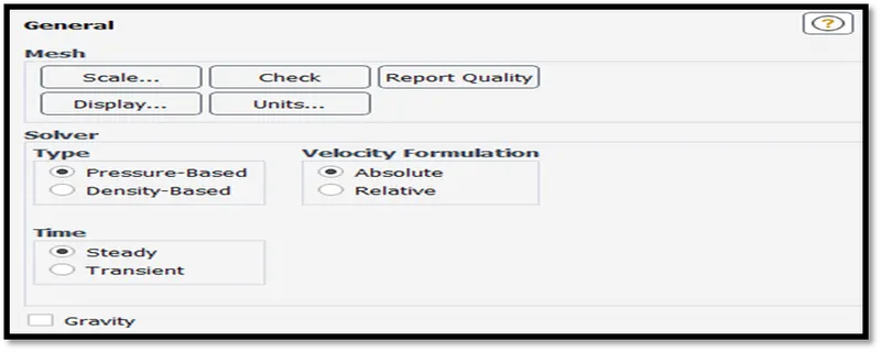
Pressure based solver and a steady state approach is chosen for the simulation.
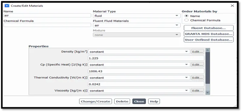
The density of the fluid (air) is set to 1.225kg/m3 with viscosity set as a constant.
The velocity of the fluid at inlet also checked with 1m/s 3.5m/s and 5m/s for the refined mesh.
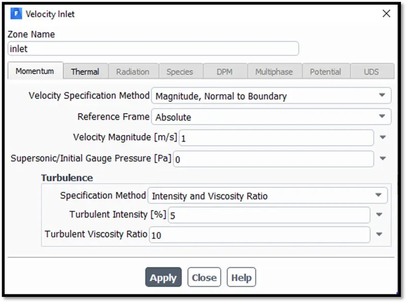
The temperature is set to 300K for the hot inlet fluid.
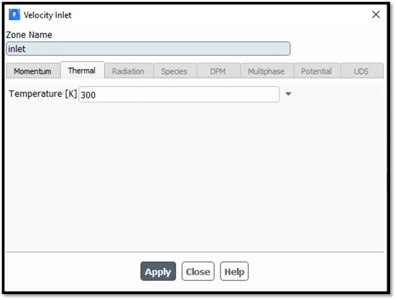
The gauge pressure is mentioned as 0 i.e., 1 atm pressure.
The convective heat transfer coefficient is set to 25.32 W/m2 K for the outer convective wall of processor (copper) and simulations performed for different velocities for case ‘C’ (refined mesh) only.
All other settings are kept as default.
Hence, for the processor (solid) a source term is mentioned to trigger heat generation by the processor solid body. This heat has to be dissipated for which the simulation is performed. The number of energy sources is set to 1 (i.e., processor) and the power per unit volume or the power density is set to 15625000 W/m3.
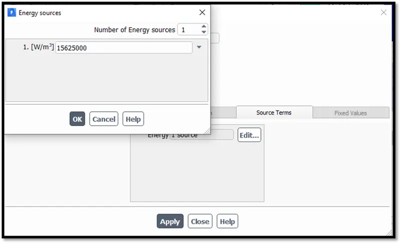
Fig: Energy source term specified for processor – Power Density is set to 15625000W/m3
The area of the processor is 64 x 10-9m3. The heat generation rate becomes 1W / 64 x 10-9m3, which is equal to 15625000W/m3. The conjugate heat transfer approach by mentioning the heat flux value is applied only to case ‘C’.
The calculation was initialized using the “hybrid initialize” option and run for 250 iterations. The solution was converged around 28% calculation time at 73rd iteration for the base mesh simulation. The calculation time was similar for the refined mesh as well.
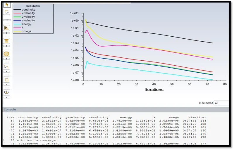
Fig: Residual plot of base mesh, solution converged at 73rd iteration
RESULTS
250 iterations were mentioned for each model. Calculation solution for case ‘A’, case ‘B’ and case ‘C-i’ converged between 70-80 iterations.
Here, the simulation is performed to display contours for the base mesh (case ‘A’), refined mesh (case ‘B’) and results obtained for a conjugate approach for different velocities (case ‘C’) are recorded.
Case ‘A’
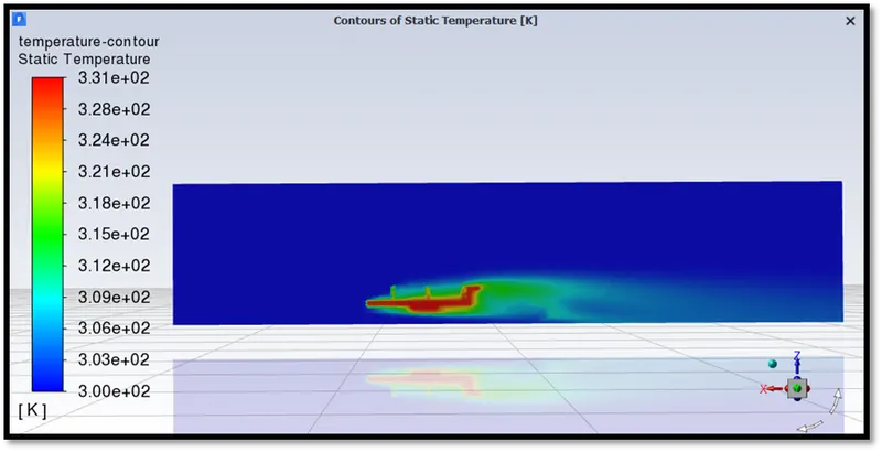
Fig: Temperature contour of XZ plane – case ‘A’
We can see that as the processor is generating heat, the contour produces an image which displays the heat getting carried away by the air flowing at 1m/s. A maximum temperature of 331K is simulated at the processor section by looking at the contour.
Case ‘B’
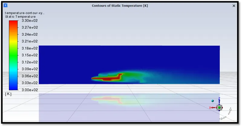
Fig: Temperature contour of XZ plane – case ‘B’
For the refined mesh, the temperature contour shows a maximum temperature of 330K recorded at the processor section for velocity at inlet being 1m/s.
Case ‘C’
- Inlet velocity is set to 1 m/s
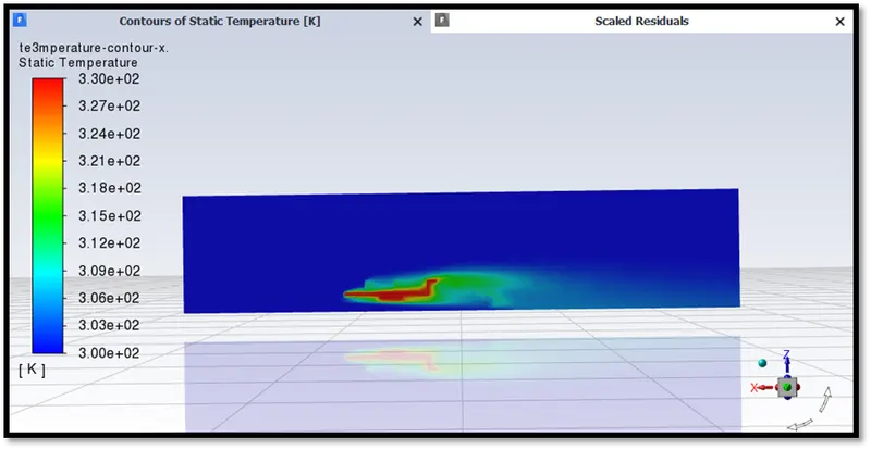
Fig: Temperature contour of XZ plane – case ‘C-i’
A temperature distribution for this case is more or less the same as case ‘B’ after specifying the heat flux at the processor walls as 25.32W/m2.
- ii) Inlet velocity is set to 3.5 m/s
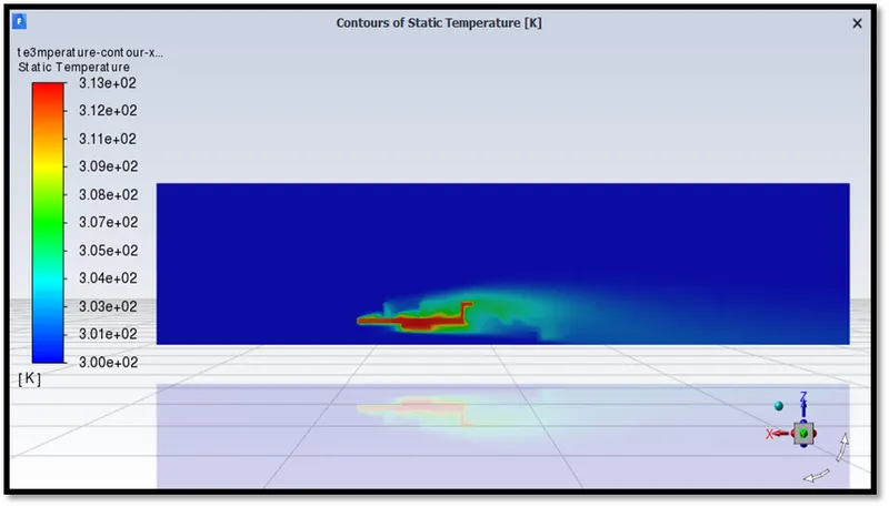
Fig: Temperature contour of XZ plane – case ‘C-ii’
For all cases, it is observed that the potential hotspots of the model are the processor and fins section helping to dissipate heat as air flows around these bodies.
The images as follows show the variation of temperatures at the hotspots at different plane sections.
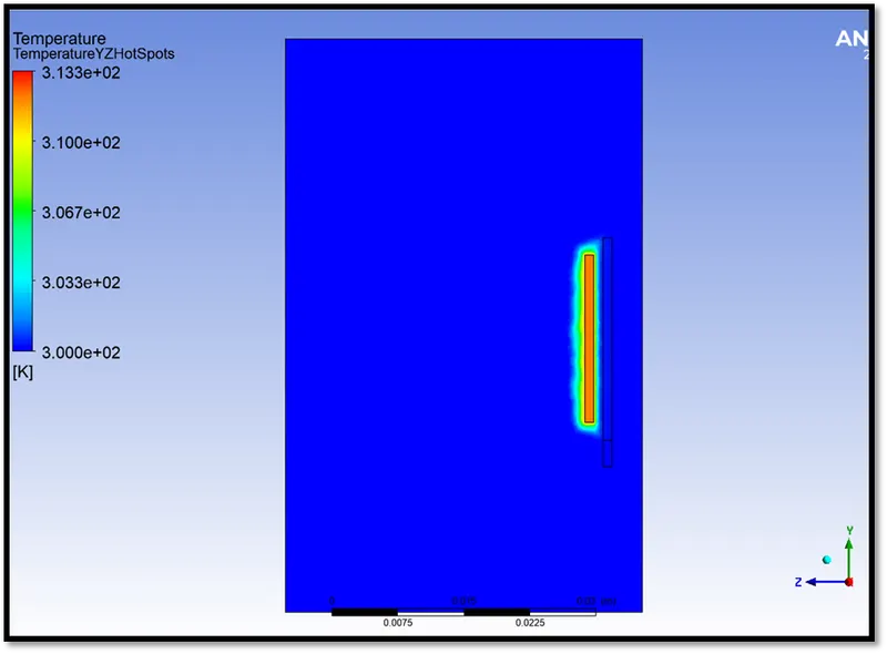
Fig: Section plane YZ – I (near inlet before processor)
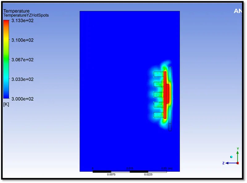
Fig: Section plane YZ – II (at processor)
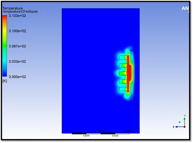
Fig: Section plane YZ – III at end of processor
From the above images I, II and III, it is observed that near the processor the heat generation region, the temperature is close to 310K (maximum temperature) and as the fluid passes over the fins, heat dissipation is achieved to reduce the temperature and keep the processor at optimum working conditions.
iii) Inlet velocity is set to 5 m/s
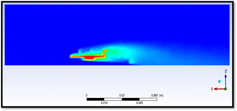
Fig: Temperature contour of XZ plane – case ‘C-iii’ (CFD-Post)
The minimum and maximum temperatures of the above contour are in the range 299.999K and 310.681K.
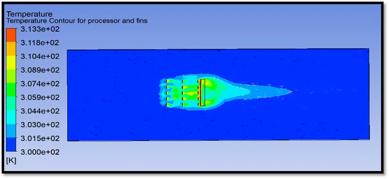
Fig: XY plane view coloured by temperature contour at fins – case C-ii
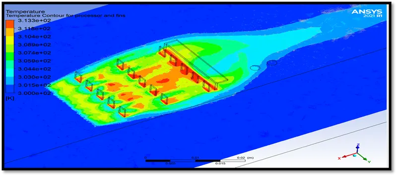
Fig: XY plane view of case C-ii, plane located just above the processor
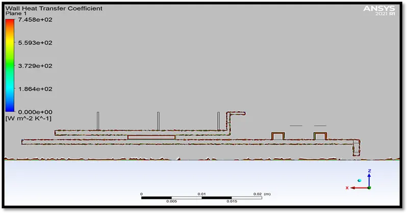
Fig: Wall Surface Heat Transfer Coefficient Contour - XZ plane – case ‘C-iii’
A table below shows the variation of all the three cases for temperature values and descriptive images for convective heat transfer coefficients at the processor walls.
|
Temperature Values for All Cases |
||||
|
Case |
Velocity (m/s) |
Temperature of graphics card enclosure (base) (K) |
Temperature of processor (K) |
Temperature of fins (K) |
|
A |
1 |
308.97007 |
330.50747 |
329.77867 |
|
B |
1 |
308.99886 |
329.75589 |
329.05276 |
|
C - i |
1 |
308.95178 |
329.24099 |
328.20592 |
|
C - ii |
3.5 |
302.2785 |
312.79968 |
312.53866 |
|
C - iii |
5 |
301.53157 |
310.16026 |
309.91606 |
It is observed that as the velocity increases by 2.5m/s between cases ‘C-i’ and ‘C-ii’ (increase by 250%), the temperature decrease is by 4.7736%. An increase by 4 m/s from case ‘C-i’ (increase by 400%) provides a further decrease in temperature by 5.5726%.
The solutions for cases C-ii and C-iii have completed 250 iterations and no message of convergence was found as the values take a longer time to reach the convergence criteria for the steady state simulation. This is because of the increase in velocity and it’s effect on the values to achieve convergence. The parameters to tend to zero are affected by the increase in velocity.
CONCLUSION
The simulation was performed using the k-w turbulence model for all cases. Case C - i, ii and iii were performed w=by specifying the heat flux for a CHT approach. The least processor temperature at 309.91K was obtained with an inlet velocity of 5m/s for case C-iii. A difference percentage of 5.732% was obtained between cases C-I and C-iii, i.e., a temperature drop by 5.57%. The difference percentage between the base mesh (case ‘A’) and refined mesh (case ‘B’) for a 1m/s air velocity inlet is found to be 0.22% only.
References
http://journalarticle.ukm.my/14309/1/17.pdf
[2] Internet sources and information
[3] Wikipedia website link - https://en.wikipedia.org/wiki/Fluid_dynamics