Week 3.5 - Deriving 4th order approximation of a 2nd order derivative using Taylor Table method
Given function:
f = exp(x)*cos(x)
2nd order derivative of the function
f'' = -2*exp(x)*sin(x)
1) Developing Taylor Table for the Forward Differencing Scheme Approximation method
For FDS, f = (af(x) + bf(x+dx) + cf(x+2dx) + df(x+3dx) + ef(x+4dx))/(dx^2)
Table:
2) Developing Taylor Table for the Backward Differencing Scheme Approximation method
For BDS, f = (af(x) + bf(x-dx) + cf(x-2dx) + df(x-3dx) + ef(x-4dx))/(dx^2)
Table:
3) Developing Taylor Table for the Central Differencing Scheme Approximation method
For CDS, f = (af(x-2dx) + bf(x-dx) + cf(x) + df(x+dx) + ef(x+2dx))/(dx^2)
Table:
Coefficient for all three approximation methods will be calcualted in MATLAB only.
Code:
Main Code:
clear all
close all
clc
%inputs
x=pi/3;
%stepsize range
dx=linspace(pi/4,pi/400,2000);
%Analytical derivative
%f(x) = exp(x)*cos(x)
%f'(x)=(exp(x)*cos(x)-(exp(x)*sin(x)=exp(x)*(cosx-sinx)
%Double derivative f" = -2*exp(x)*sin(x)
analytical_derivative = -2*exp(x)*sin(x);
%Skewed right-sided(4th order approimation)
%Solving for the coefficients
A=[1 1 1 1 1 1;0 1 2 3 4 5; 0 1/2 4/2 9/2 16/2 25/2; 0 1/6 8/6 27/6 64/6 125/6; 0 1/24 16/24 81/24 256/24 625/24; 0 1/120 32/120 243/120 1024/120 3125/120];
B=[0;0;1;0;0;0];
x_r=inv(A)*B;
%Skewed left-sided(4th order approimation)
%Solving for the coefficients
C=[1 1 1 1 1 1;0 -1 -2 -3 -4 -5; 0 1/2 4/2 9/2 16/2 25/2; 0 -1/6 -8/6 -27/6 -64/6 -125/6; 0 1/24 16/24 81/24 256/24 625/24; 0 -1/120 -32/120 -243/120 -1024/120 -3125/120];
D=[0;0;1;0;0;0];
x_l=inv(C)*D;
%central differencing(4th order approimation)
%Solving for the coefficients
E=[1, 1, 1, 1, 1; -2, -1, 0, 1, 2; 4/2, 1/2, 0, 1/2, 4/2; -8/6, -1/6, 0, 1/6, 8/6; 16/24, 1/24, 0, 1/24, 16/24];
F=[0;0;1;0;0];
x_c=E^-1*F;
%Anonymous Function
f=@(x) exp(x).*cos(x);
%numerical derivative
right_difference=(x_r(1)*f(x)+x_r(2)*f(x+dx)+x_r(3)*f(x+2.*dx)+x_r(4)*f(x+3.*dx)+x_r(5)*f(x+4.*dx)+x_r(6)*f(x+5.*dx))./(dx.^2)
left_difference=(x_r(1)*f(x)+x_r(2)*f(x-dx)+x_r(3)*f(x-2.*dx)+x_r(4)*f(x-3.*dx)+x_r(5)*f(x-4.*dx)+x_r(6)*f(x5.*dx))./(dx.^2)
cent_difference=(x_c(1)*f(x2.*dx)+x_c(2)*f(x1.*dx)+x_c(3)*f(x)+x_c(4)*f(x+dx)+x_c(5)*f(x+2.*dx))./(dx.^2)
%absolute error
error_r=abs(analytical_derivative-right_difference);
error_l=abs(analytical_derivative-left_difference);
error_c=abs(analytical_derivative-cent_difference);
error=[error_r;error_l;error_c];
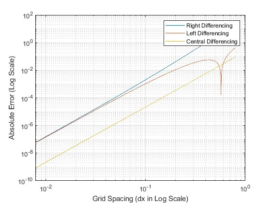
figure(1)
loglog(dx,error_r)
grid on
hold on
loglog(dx,error_l)
loglog(dx,error_c)
ylabel('Absolute Error (Log Scale)')
xlabel('Grid Spacing (dx in Log Scale)')
legend('Right Differencing','Left Differencing','Central Differencing')
RESULTS: