Week 2 - Flow over a Cylinder.

Numerical simulation of the flow over a cylinder at different Reynolds numbers.

Objective-

To simulate the flow over a cylinder at different Reynolds number and explain the formation of Karman Vortex Street. Also, to calculate the drag and lift coefficient over the cylinder.

Introduction-

Flow over bodies that are immersed in a fluid includes the flow of air around airplanes, automobiles, and falling snowflakes or the flow of water around submarines and fish. In these situations the object is completely surrounded by the fluid, and the flows are termed external flows.

When anybody moves through a fluid, an interaction between the body and the fluid occurs; this effect can be described in terms of the forces at the fluid-body interface.

In fluid dynamics, a Kármán vortex street (or a von Kármán vortex street) is a repeating pattern of swirling vortices, caused by a process known as vortex shedding, which is responsible for the unsteady separation of flow of a fluid around blunt bodies.

A vortex street will form only at a certain range of flow velocities, specified by a range of Reynolds numbers (Re), typically above a limiting Re value of about 90. The (global) Reynolds number for a flow is a measure of the ratio of inertial to viscous forces in the flow of a fluid around a body or in a channel, and may be defined as a non-dimensional parameter of the global speed of the whole fluid flow.

Re = (ρuL)/μ

ρ = density of the fluid

u = flow speed

L = characteristic linear dimension

μ = dynamic viscosity of the fluid

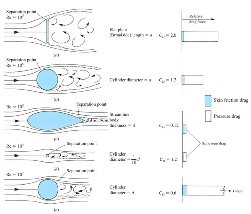
At very low values of the Reynolds number, the coefficient of drag is given by exact equations relating CD and Re. At high values of Re, the coefficient of drag becomes constant for angular bodies, whereas rather abrupt changes in CD occur for rounded bodies. All these characteristics can be seen in the following figure, where CD is plotted against Re for several axisymmetric bodies.

Strouhal Number:

In dimensional analysis, the Strouhal number (St, or sometimes Sr to avoid the conflict with the Stanton number) is a dimensionless number describing oscillating flow mechanisms. The Strouhal number is an integral part of the fundamentals of fluid mechanics.

St=f*L/U

f = frequency of vortex shedding,

L = characteristic length (for example, hydraulic diameter or the airfoil thickness)

U = flow velocity.

Vortex shedding-

In fluid dynamics, vortex shedding is an oscillating flow that takes place when a fluid such as air or water flows past a bluff (as opposed to streamlined) body at certain velocities, depending on the size and shape of the body. In this flow, vortices are created at the back of the body and detach periodically from either side of the body forming a Kármán vortex street. The fluid flow past the object creates alternating low-pressure vortices on the downstream side of the object. The object will tend to move toward the low-pressure zone.

If the bluff structure is not mounted rigidly and the frequency of vortex shedding matches the resonance frequency of the structure, then the structure can begin to resonate, vibrating with harmonic oscillations driven by the energy of the flow.

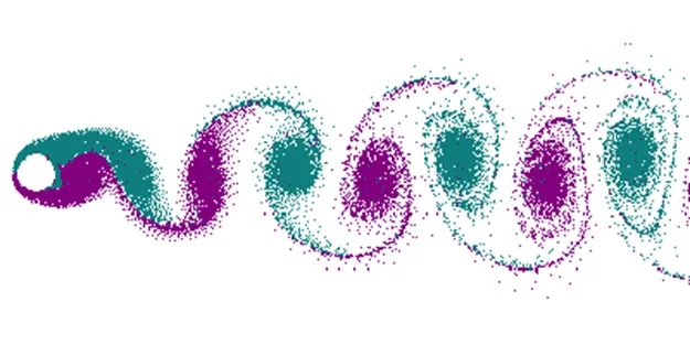
Vortex shedding behind a circular cylinder. Here, the flows on the two sides of the cylinder are shown in different colors, to show that the vortices from the two sides alternate.

Procedure-

A 2 dimensional cylinder was modeled to study the Karman vortex street with respect to the Reynolds number using ANSYS-Fluent. The density and viscosity of the fluid was maintained as 1 kg/m3 and 0.05 kg/m.s. The problem was simulated under the steady and unsteady state condition. The flow was maintained as laminar boundary layer condition. The drag and lift coefficient was found under varying Reynolds number (i.e. 10,100,1000,10000 & 100000).

Modelling-
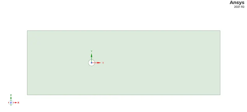
In space claim, we have to make a circle and flow boundary as per given problem statement as shown below-

Meshing-

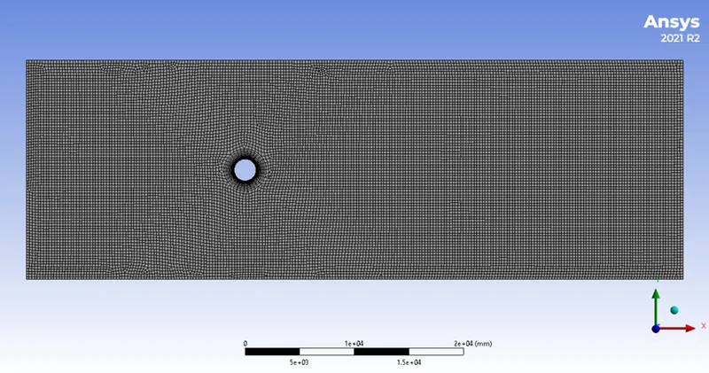
Here, the mesh size was 250mm and since we want to capture the properties near the cylinder so we need to add inflation layer. The first layer height can be calculated for desired Y+ value analytically which requires value of free stream velocity, density of fluid, dynamic viscosity and characteristic length.

Pre-Processing and Solver Setting:

Problem Setup>Viscous>laminar.

Problem Setup>materials>create new material (user material)> give 1 kg/m3 and 0.05 kg/m.s. as density and viscosity respectively.

Problem Setup>Boundary conditions: Select cell zone conditions as fluid and the material name as user material.

For Inlet, select type as velocity-inlet, click edit and enter the velocity as 2.5 m/s under the Momentum tab. So, that the Reynolds number will be 100. And select the pressure-outlet for the outlet, since it is open to the atmosphere.

Create a point at an X distance of 8 m to study the vertex flow. To generate reports, for example to create a vertex average. Click under Reports>Definitions>new> surface report>vertex average, then select variable as velocity and surfaces as monitor point.

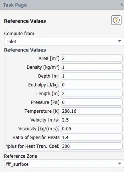
Select the method as Simple Scheme method. In computational fluid dynamics (CFD), the SIMPLE algorithm is a widely used numerical procedure to solve the Navier-Stokes equations. SIMPLE is an acronym for Semi-Implicit Method for Pressure Linked Equations.

To solve the problem, select Hybrid Initialization under the solution tab.

Results-

Part1-

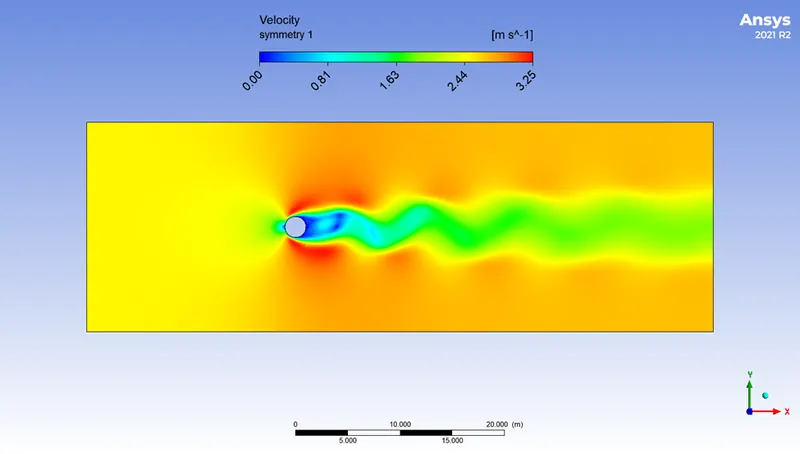
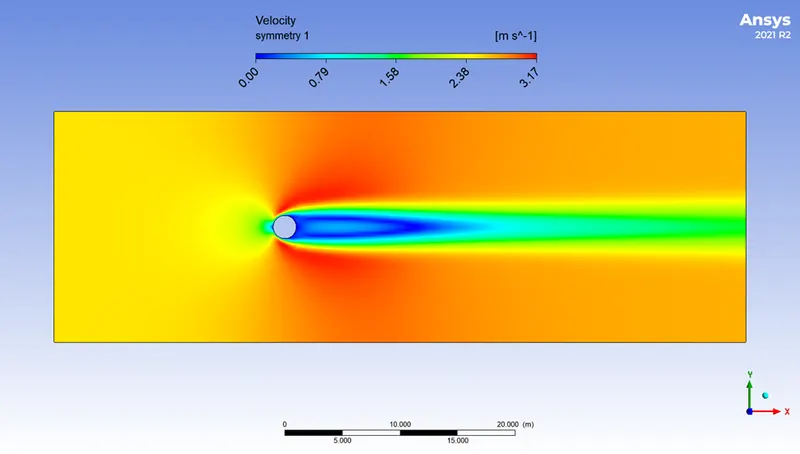
Simulation of flow over a cylinder as velocity contour under steady and unsteady flow for Re = 100 is shown below -

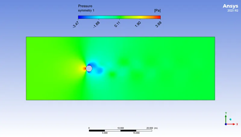
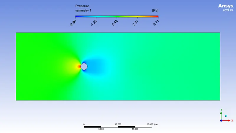
Simulation of flow over a cylinder as pressure contour under steady and unsteady flow for Re = 100 is shown below -

Plot between drag and Strouhal number for steady and unsteady flow is shown below-

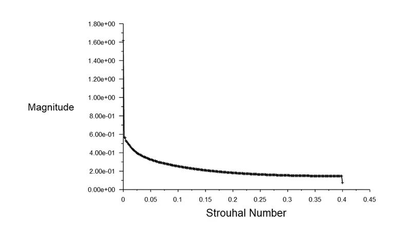
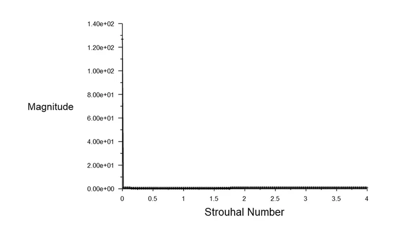
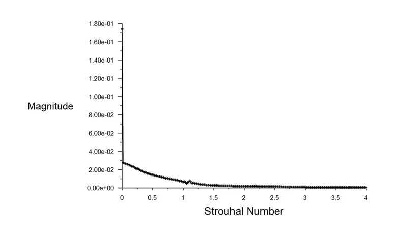
As you can see from the above plots, under steady and unsteady conditions the Strouhal number is about 0.4 and 4 respectively.

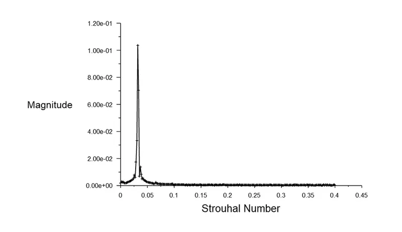
Plot between lift and Strouhal number for steady and unsteady flow is shown below-

Part 2-

The scaled residual plots for different Reynolds number of 10, 100, 1000, 10000, 100000 are shown below-

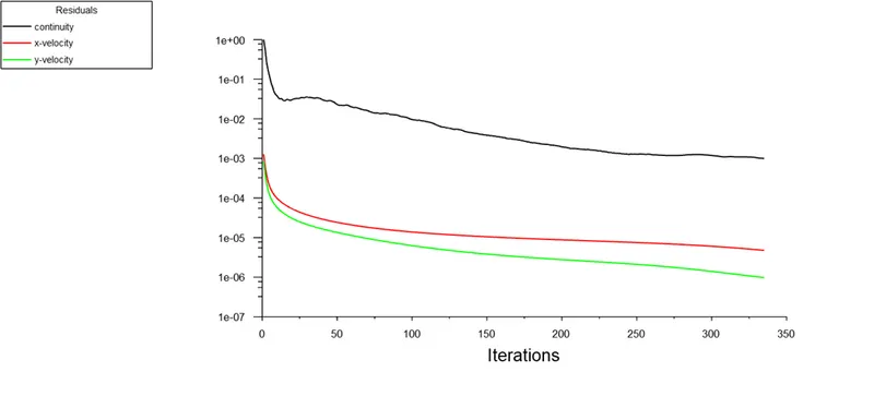
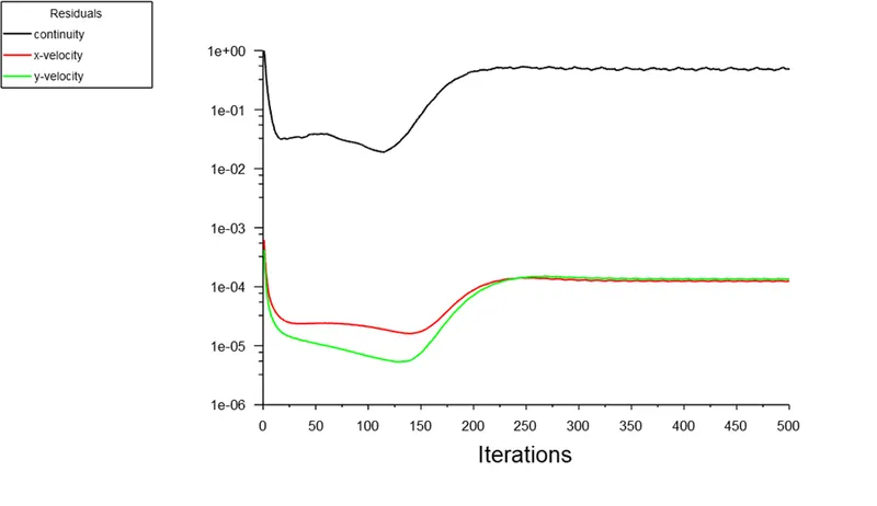
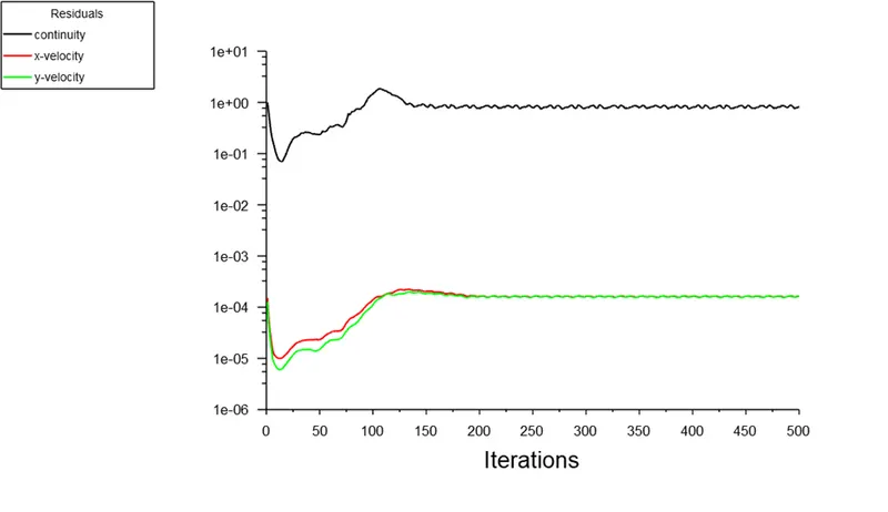
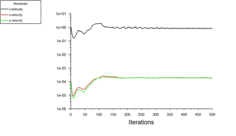
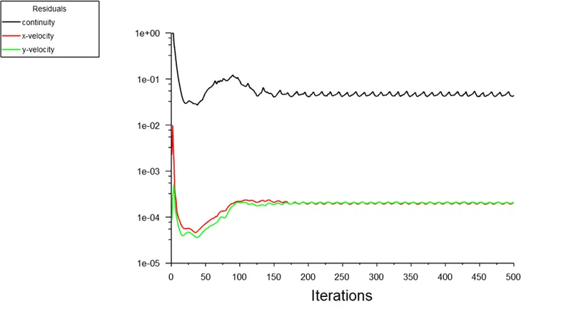
From all the above residual plots for different Reynolds numbers, we can see that the solution converged for all the solutions after some hundreds iterations.

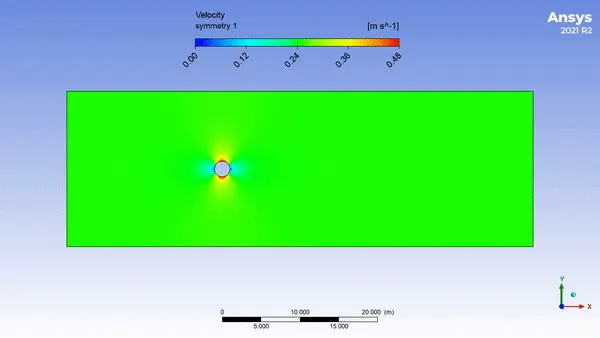
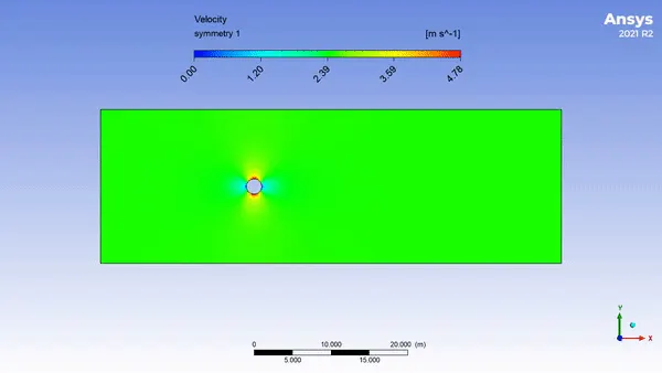
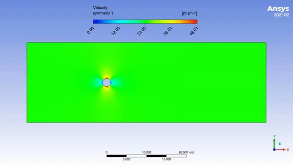
The velocity contour profile for different Reynolds number of 10, 100, 1000, 10000, 100000 are shown below-

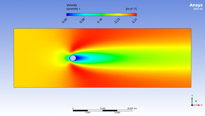
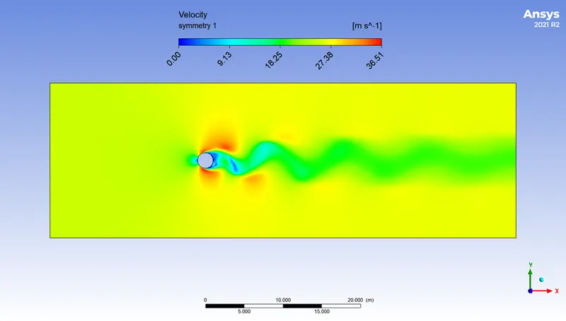
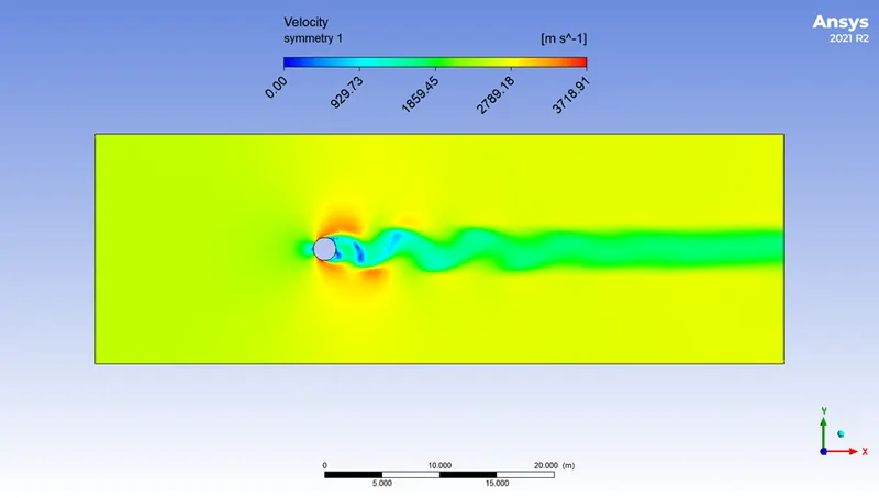
As you can see in the above velocity contours, as the Reynolds number increases, there is formation of wake regions after the cylinder. Also there is formation of vortex shedding which can be seen above contours.

The velocity animation videos for different Reynolds number of 10, 100, 1000, 10000, 100000 are shown below-

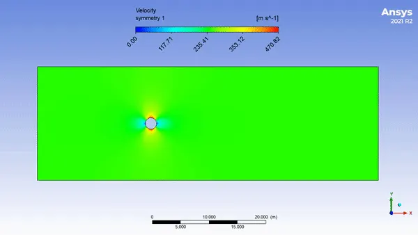
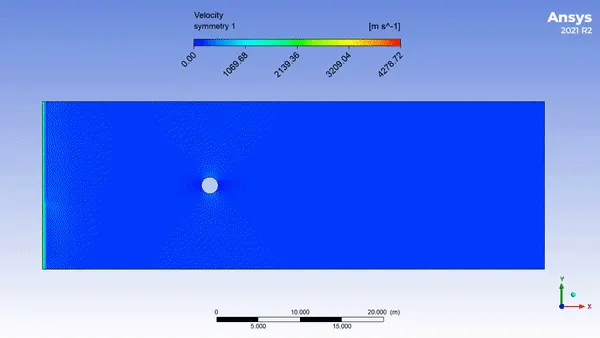
The pressure contour profile for different Reynolds number of 10, 100, 1000, 10000, 100000 are shown below-

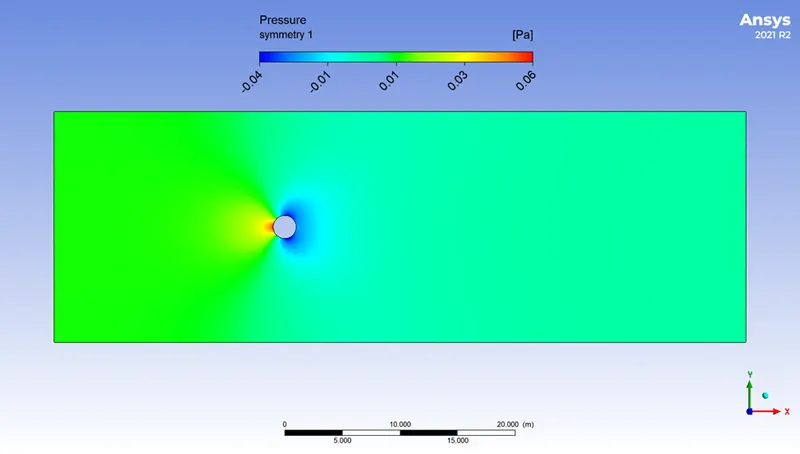
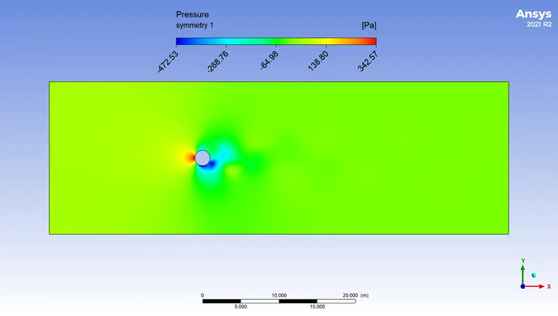
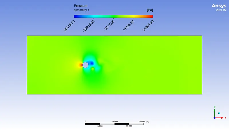
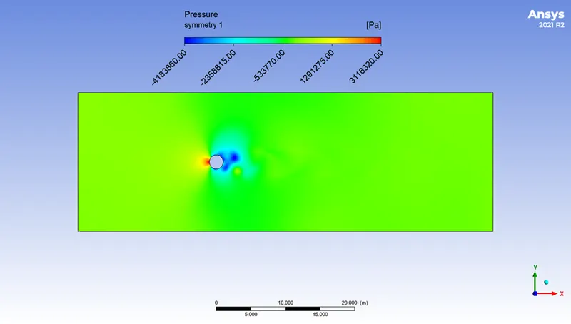
From the above pressure contours, you can see there is negative pressure region above the cylinder and positive pressure region below the cylinder. Due to this pressure gradient, lift phenomenon happens on the cylinder.

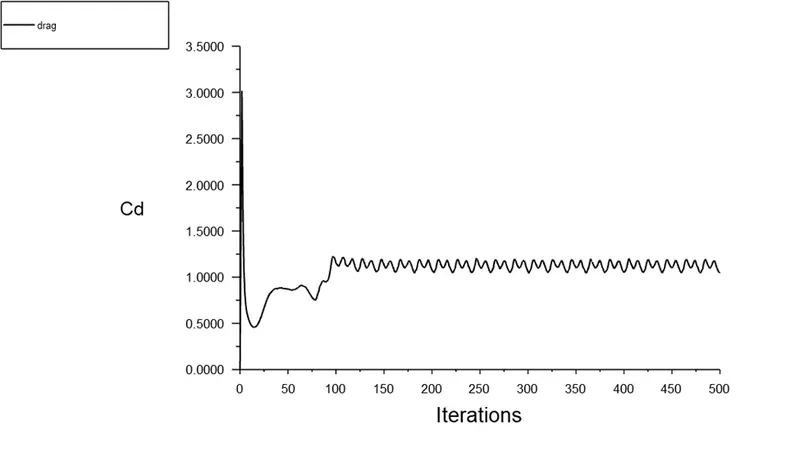
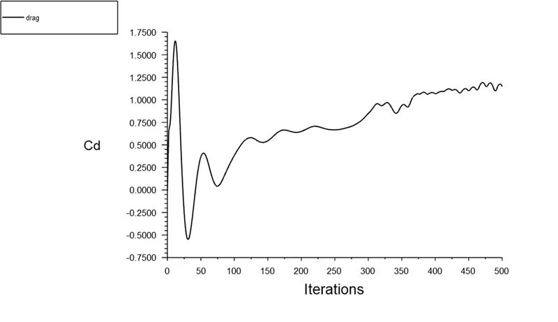
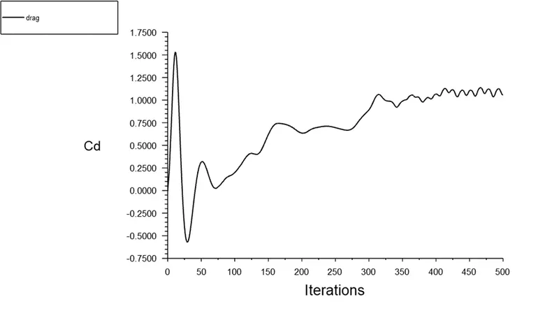
The drag coefficient plot for different Reynolds number of 10, 100, 1000, 10000, 100000 are shown below-

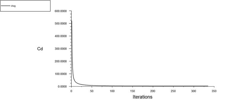
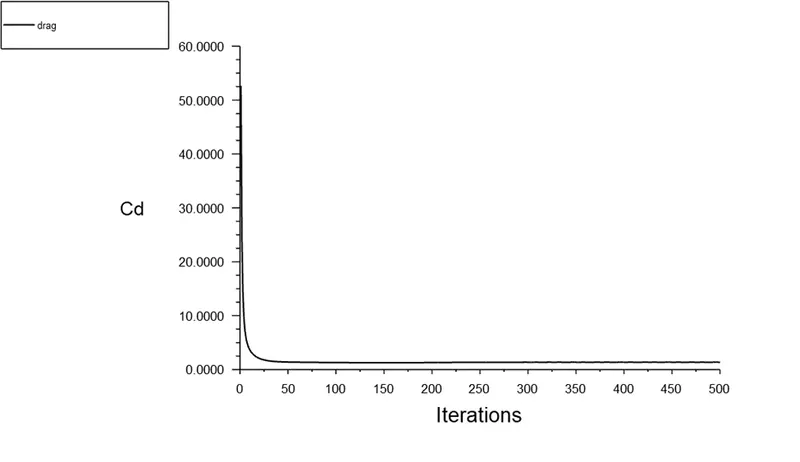
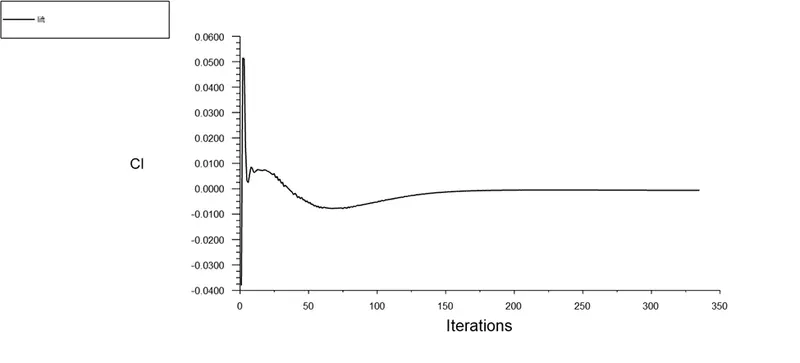
The lift coefficient plot for different Reynolds number of 10, 100, 1000, 10000, 100000 are shown below-

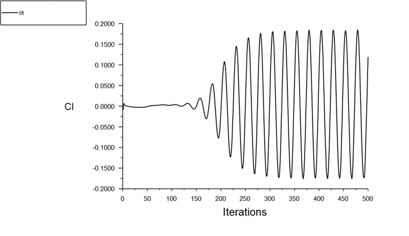
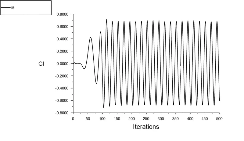
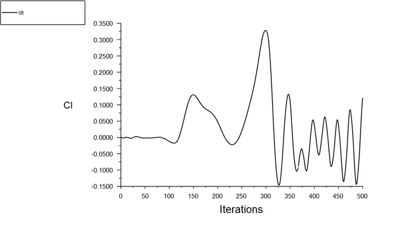
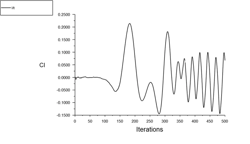
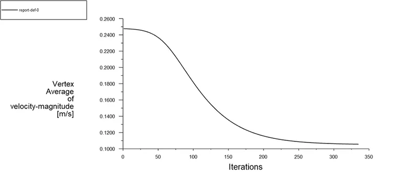
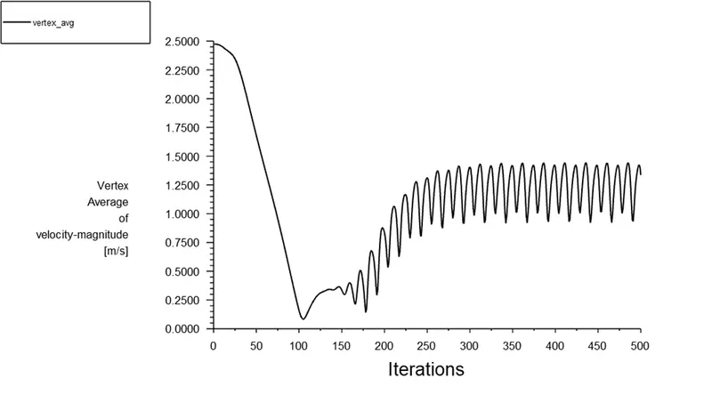
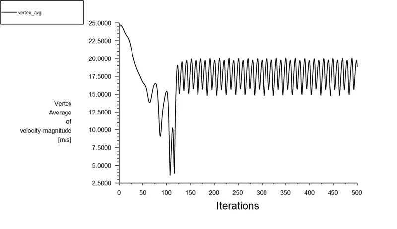
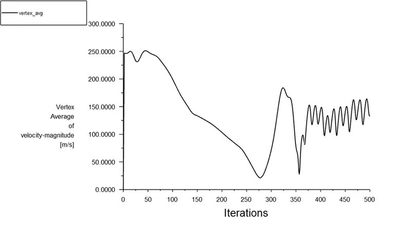
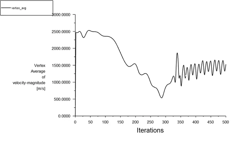
The plot for showing vortex shedding behind the cylinder can be shown by making a point behind the cylinder and making vertex average plot at that point. The plot of vertex average of velocity magnitude for different Reynolds number of 10, 100, 1000, 10000, 100000 are shown below-

Conclusion-

Reynolds Number	Drag coefficient	Lift coefficient
10	1.336573	-0.0006346941
100	1.362236	0.1751113
1000	1.055247	-0.6080006
10000	1.14779	0.1209718
100000	1.059371	0.06714469

For Reynolds number 100, we can calculate the error in our drag and lift coefficient by comparing it with a reference paper which is given below.

The error in drag and lift coefficient was found to be 2% and 2.2% respectively.

Reference Research Paper:-

https://www.sciencedirect.com/science/article/pii/S0307904X08000243