Week 6 - CHT Analysis on a Graphics card

Conjugate Heat Transfer analysis on a graphics card

Objective-

To perform a steady-state conjugate heat transfer analysis on a model of a graphics card.

Introduction-

Conjugate heat transfer is defined as the heat transfer between two domains by exchange of thermal energy. For a system the thermal energy available is defined by its temperature and the movement of thermal energy is defined by its heat flux through the outer walls. Heat transfer in solid happens through conduction and walls by convection and in liquid phase through convection.

CHT provides the temperature prediction and the hotspot regions at the solid-fluid interface and we can also predict the heat transfer accurately for example- Conduction through solids, convection through fluid, and thermal radiation. It also provides the velocity and pressure distribution of fluid moving inside the solid. We can also use CHT in design optimization for improvement for heat transfer and cooling capacity.

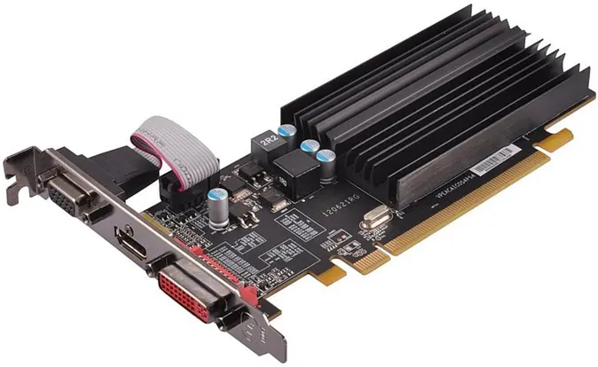
A video card (also called a graphics card, display card, graphics adapter, or display adapter) is an expansion card that generates a feed of output images to a display device (such as a computer monitor). Most video cards are not limited to a 6-inch simple output. Their integrated graphics processor can perform additional processing, removing this task from the central processor of the computer.

Procedure-

Here, we have model of a graphics card, on which we have to perform pre-processing for meshing.

Modelling-

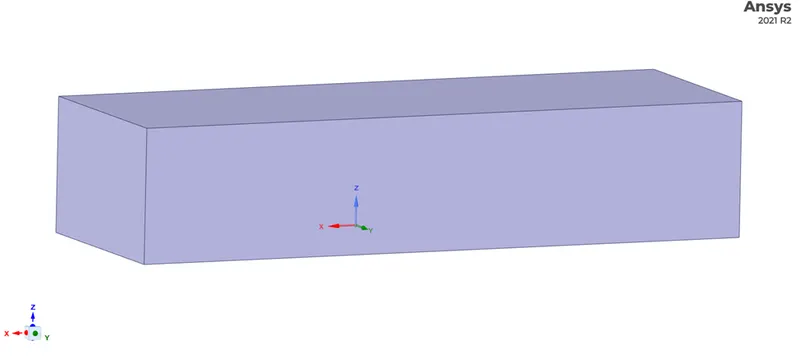
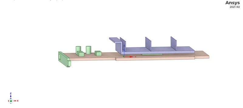
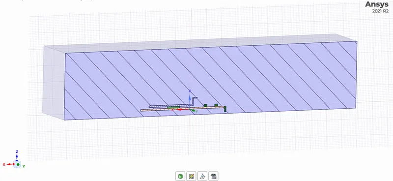
Here, we have to use share topology tool for correct information transfer between the nodes at the boundary of the enclosure and graphics card. Below images show the enclosure, graphics card and cut section of the model respectively.

Meshing-

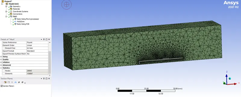
Case 1- Here, base mesh size is 6mm and mesh size of fins, processor and PCB is kept 1mm by using body sizing tool. Below image shows the meshed model-

Total elements = 158897

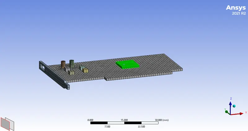
Now, we have name the front face of enclosure as inlet, back face as outlet and side faces as symmetry. Below image shows the processor and is named accordingly-

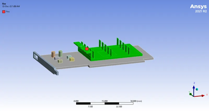
Below image shows the fins and is named accordingly-

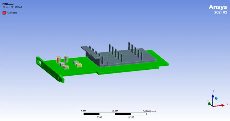
And lastly below image shows the PCB and is named accordingly-

Pre-Processing and Solver Setting:

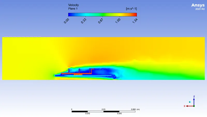
For case 1 we are taking inlet velocity as 1m/s.

Here we are using solver type as pressure based and steady solver. Then we are selecting viscous model as K-omega SST model. The solution method scheme here is coupled method.

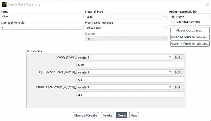
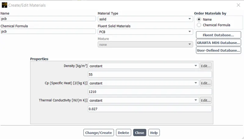
Now, to add material, copy aluminum (default solid material) in fluent database then it gives option to add new material. Then, add two materials, one for processor and other for PCB. Below table shows the properties of the materials-

Part	Material	Thermal Conductivity (W/m.k)	Specific heat capacity (J/Kg.K)	Density (Kg/m3)
Fin	Aluminum	202.4	871	2719
Processor	Silicon	153	703	2330
PCB	Polystyrene	0.027	1210	55
Heat transfer fluid	Air	0.0242	1006.43	1.225

Below images show the inputs to add materials aluminum and silicon-

Then under cell zone conditions, change the zones into their respective type like PCB is solid type, processor is solid type.

Now to calculate the heat generated by the processor-

Size of processor - 8mm X 8mm X 1mm

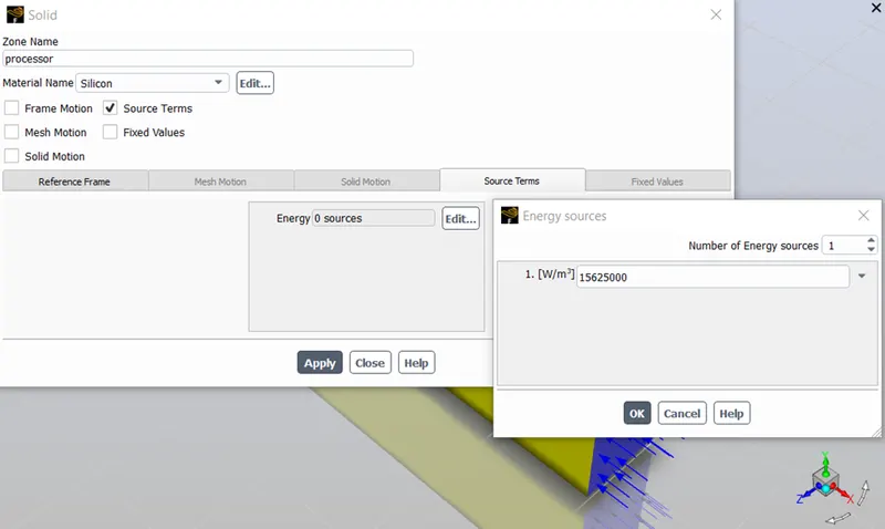
Assuming the heat dissipation of the processor as 1W, the heat generated by the processor will be 1562500 W/m³ (heat dissipation/volume of processor).

Now, for processor, select source term since it is the source of heat generation, then under it increase number of energy source to 1 and input 1562500W/m3 as heat generated by it.

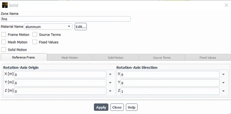
For fins change the type to solid and change the material to aluminum. Below image shows the input -

Now, under boundary conditions, change the inlet velocity magnitude to 1m/s.

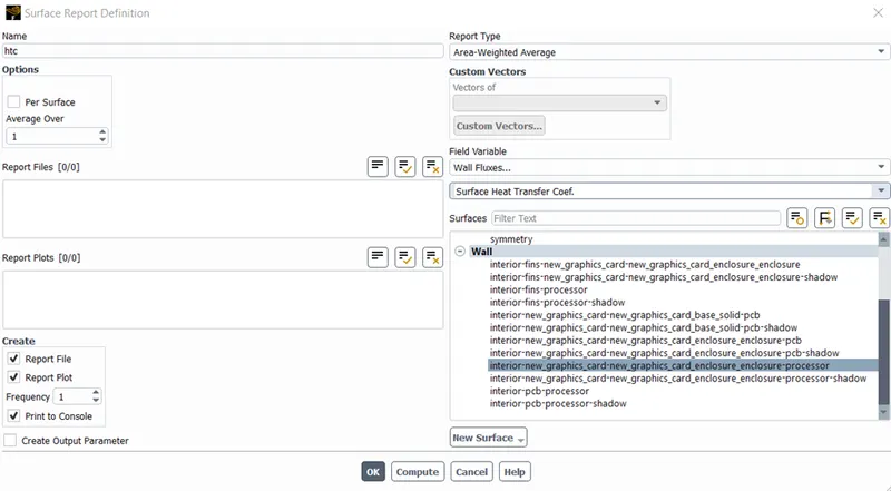
After this, we have to add report to plot heat transfer coefficient at the exposed surface of the processor. Below image shows the report creation tab-

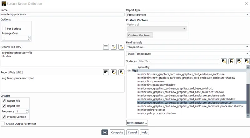
Now, we have to add two more reports describing the average and maximum temperature of the processor. Below image shows the report generation of maximum temperature of the processor-

Now, initialize the solver using hybrid initialization and then run the solver for 200 iterations.

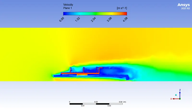
Case 2- We are taking inlet velocity of air as 3m/s in this case while other settings and inputs are same as the case 1.

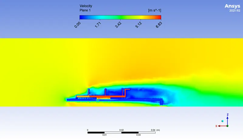
Case 3- We are taking inlet velocity of air as 5m/s in this case while other settings and inputs are same as the case 1. Then we will compare the maximum temperature and heat transfer coefficient in each cases.

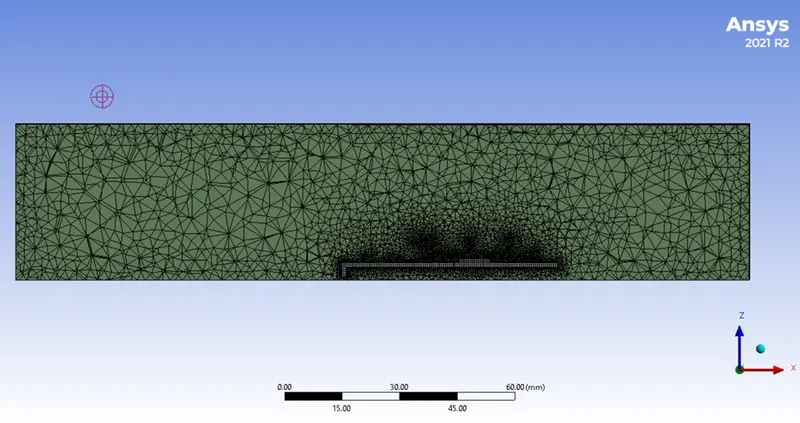
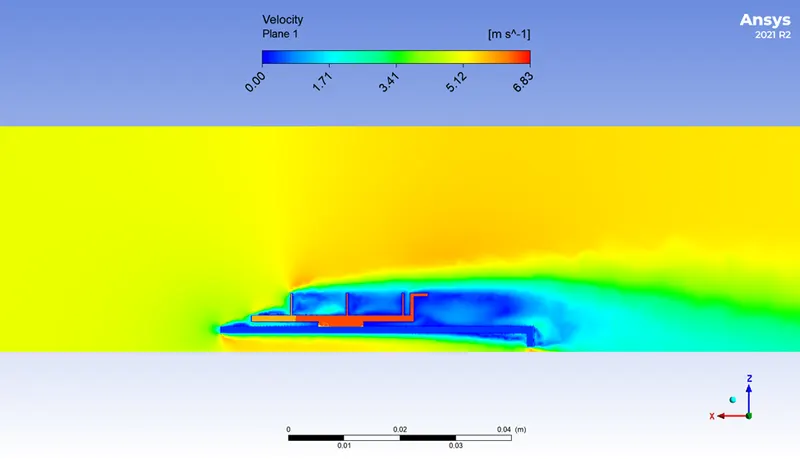
Case 4- In this case we are changing the mesh size for mesh independent study. Here, we are taking base mesh size as 3mm while fins, processor and PCB as 0.5mm. The inlet velocity of the air will be 5m/s.

Total elements = 591030

Below image shows the meshed model-

Result-

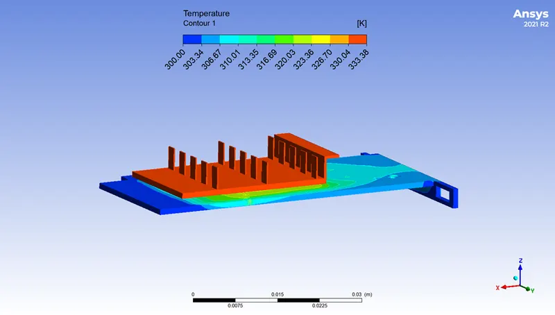
Below image shows the temperature distribution on the graphics card for case 1-

The temperature contour for cases 1, 2, 3 and 4 are shown below-

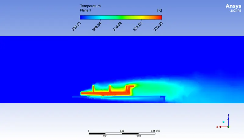
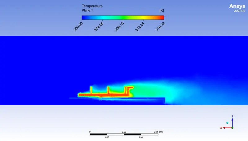
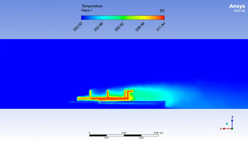
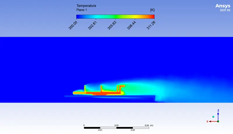
From the above images you can see the decrease in the maximum temperatures of the processor and fins as the inlet velocity of air increases.

The velocity contour for cases 1, 2, 3 and 4 are shown below-

The velocity vector for case 3 and 4 is shown below-

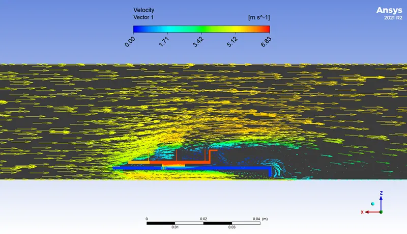
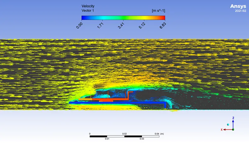
Here, you can see the difference in the velocity vector details around the graphics card due the finer mesh size in case 4.

The heat transfer coefficient of processor for cases 1, 2, 3 and 4 are shown below-

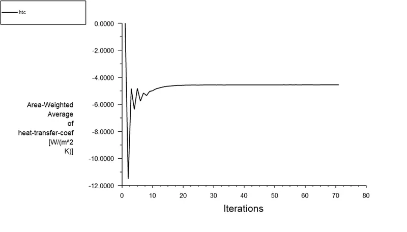
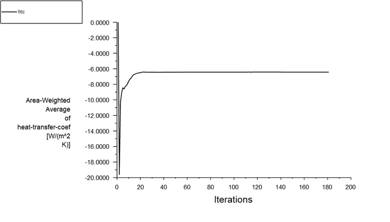
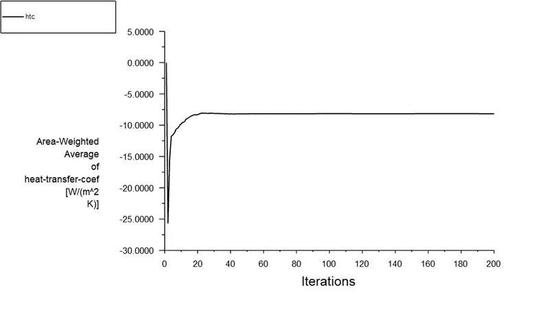
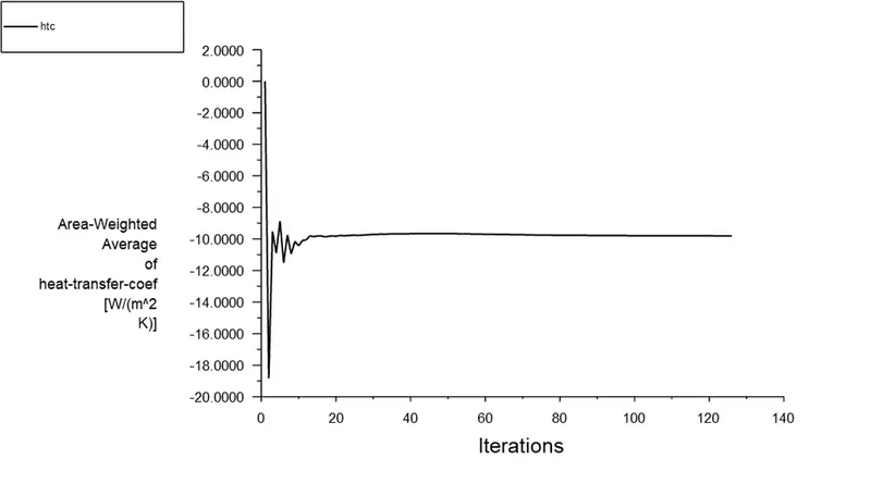
From the above plots, you can see the convergence of the solution after 30-40 iterations as the value of the heat transfer coefficient becomes constant.

Conclusion-

Below table shows the values of maximum temperature and heat transfer coefficient of processor for different cases-

Case	Velocity (m/s)	Maximum temperature (K)	Heat transfer coefficient (W/m2.K)
1	1	333.3506	4.556082
2	3	316.2839	6.422271
3	5	311.9938	8.167753

The above table shows that as the velocity increases the maximum temperature decreases and the heat transfer coefficient increases but there is not much difference in the maximum temperature for case 2 and 3.

Below table shows the mesh independent study-

Case	Base mesh size	Number of elements	Maximum temperature (K)	Heat transfer coefficient (W/m2.K)
3	6	158897	311.9938	8.167753
4	3	591030	311.2118	9.8022

As you can see in the above table, the maximum temperature is almost same in both course and fine mesh cases while there is some difference in the heat transfer coefficient value which can be attributed to the finer mesh around the graphics card which better captures the properties.