Week 3 - External flow simulation over an Ahmed body.

External flow numerical simulation on the aerodynamics of the Ahmed body using Ansys fluent

Objective-

To simulate a numerical simulation external flow of fluid over Ahmed body and calculate drag and lift coefficients.

Introduction-

Model experiments suitable for providing validation data make use of model bodies with geometries characterized by variable parameters, such as the slant angle at the back. One such body is the Ahmed body, a bluff model body of simple shape with basic aerodynamic properties of a vehicle, which has been used for many reference investigations.

Over the years, numerous studies have been conducted on the Ahmed body both computationally and experimentally using wind tunnels. Since a lot of data is available on the Ahmed body, today the geometry is primarily as a validation tool for CFD codes. The geometry of the Ahmed body is shown below:

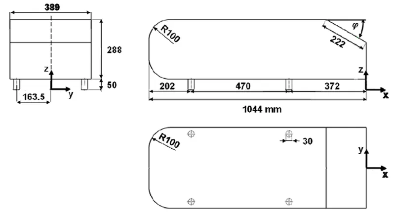
The drag force is an important factor considering fuel consumption. As the drag force increases the fuel consumption also increases which in turn becomes expensive for the car owners. As the burning of fossil fuels becomes an issue, the manufacturers are pressing for fuel-efficient cars. One of the main factors considering the car is fuel-efficient or not is the car's geometry.

Complex shaped cars are very challenging to model and it’s difficult to quantify the aerodynamic drag computationally. The Ahmed body is a benchmark model widely used in the automotive industry for validating simulation tools.

Negative pressure in the wake region-

When the air moving over the vehicle is separated at the rear end, it leaves a large low-pressure turbulent region behind the vehicle which is known as the wake. This contributes to the formation of pressure drag which affects the vehicle performance.

When the vehicle is moving at a certain velocity the fluid imparts viscous force to the vehicle as long as it is in the viscous sublayer of the boundary. When the fluid reaches the rear end of the vehicle it gets detached from the surface of the body causing negative pressure in the wake region. The movement of the fluid around the vehicles depends on the geometry of the car and the Reynolds number.

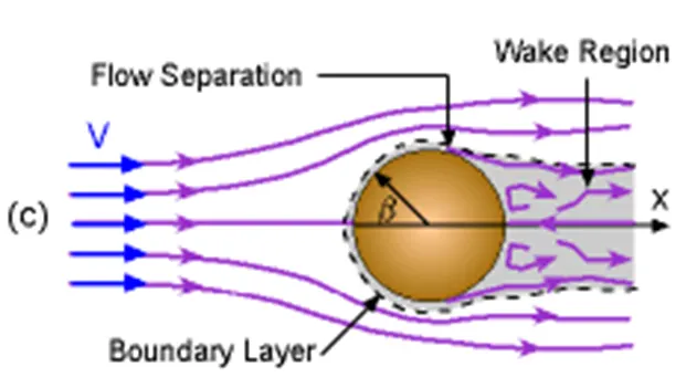
Significance of point of separation-

The point of separation will occur when there is a discontinuity in the surface or a region of the negative pressure gradient (a sharp end or rear portion of the car).

When the flow is attached to the body of the vehicle the viscous force will increase which will increase the pressure and a decrease in velocity before the rear end of the vehicle. As soon as the air encounters the sharp turn causing the velocity to decrease resulting in the negative pressure region which is in the wake region. The recirculation region happens beyond the point of separation.

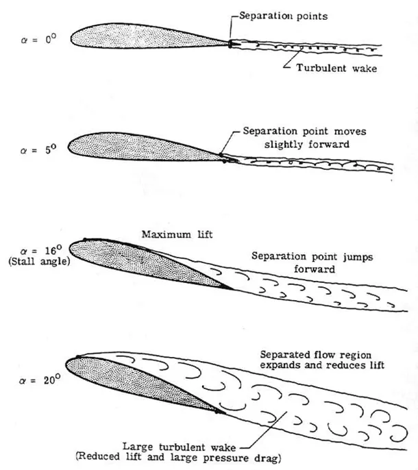
If the rate of change of pressure is large the mixing process will not occur and the boundary layer flow stops.

In order to reduce the separation of fluid from the boundary layer, it is advisable to have a smooth edge to reduce the effect of drag on the vehicle.

Procedure-

Below is the model of the Ahmed body -

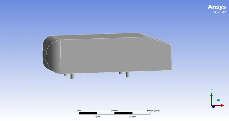
Now, before meshing and simulation, we have to create the wind tunnel or enclosure which can be accomplished in space claim. Under prepare tab, we have enclosure tool which creates enclosure according to our dimensions.

Here, we have taken following dimensions for creating the wind tunnel-

Length in front of model- 2*length of body (here, 1.044m)

Length from back of model- 5*length of body

Length from top of model- length of model

Length from sides of the model- 0.5*length of model

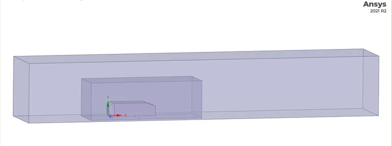
Here, we have also added one more small enclosure to focus on the important area so that we can have more precise results with less computational time. This is accomplished by giving bigger element size to the outer enclosure than the inner one which is more important to get accurate results.

Below image shows the two enclosures with the Ahmed body-

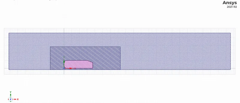
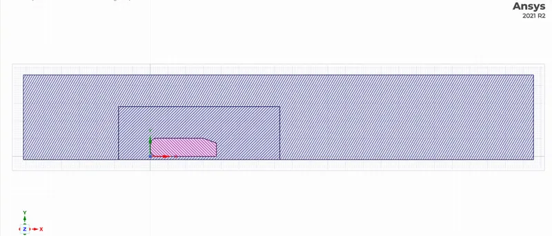
Above image shows the section image of the model. It shows the overlapping area of the two enclosures. We need to remove it so that we don't have any errors while meshing. We use interference tool to remove the overlapping surfaces. Below image shows the model after correction-

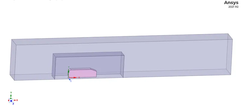
Now, since the Ahmed body is symmetric, so we don’t need to mesh the whole body for simulation. We can split the whole model by using the split body tool to delete the half of the model. Below image shows the model after using split body-

Now, we need to suppress the Ahmed body since it is not needed in the simulation and we only need the wall or space for simulation. Below image shows the model after suppressing for physics the Ahmed body-

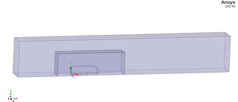
Now, since the two enclosure will have different element sizes, thus for correct information transfer between the nodes at the boundary of the two enclosures, we have to use ‘share topology’ tool. Below image shows the model after using ‘share topology’ tool-

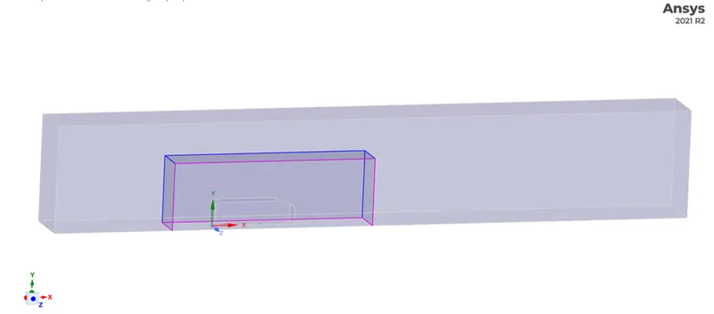
Meshing-

Case1-

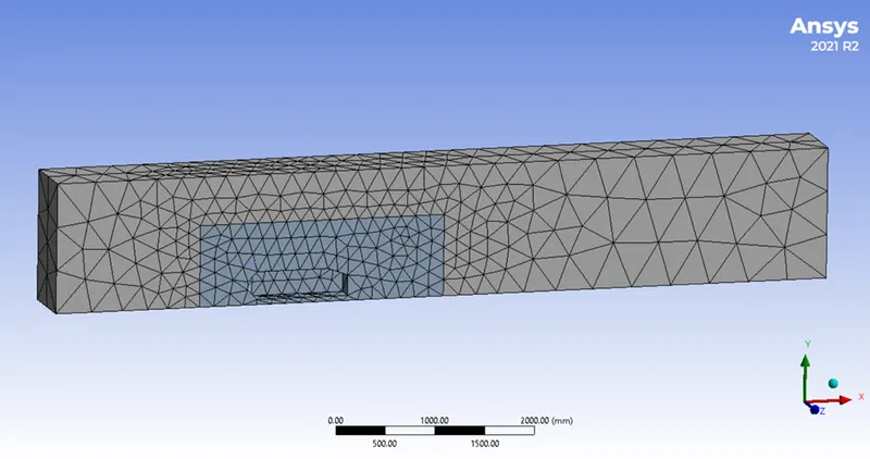
Below image shows the initial model after using the basic mesh size –

Inner enclosure = 150mm, baseline mesh = 400mm

To get better accuracy in the results-

Inserting ‘sizing’ in mesh and select the inner enclosure to give smaller element size = 40mm and make border line mesh element size = 100mm.

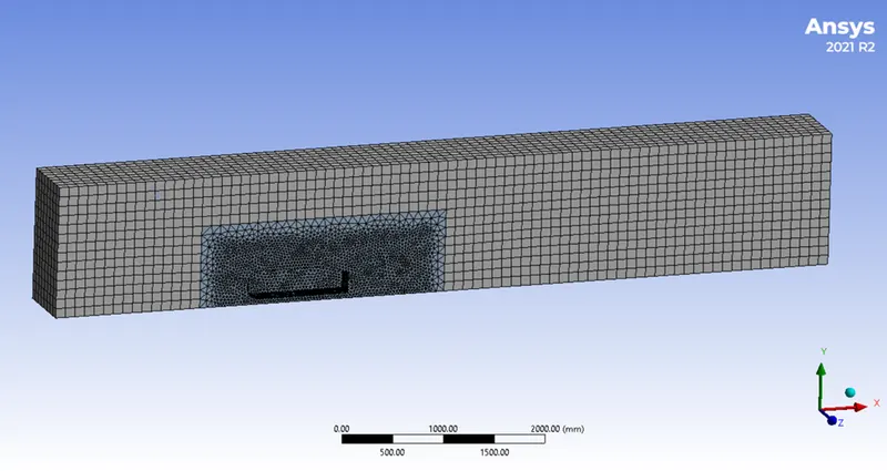
Now, since the enclosure is very big and we want to decrease the number of elements further to decrease the computing time without compromising in the accuracy in the results, so we can change the mesh type of outer enclosure by inserting ‘method’ in the ‘mesh’ and selecting ‘multi-zone’ which makes the outer enclosure element type to quad from tetra.

Below image shows the model after meshing-

Now, before adding inflation layer, we will name all the faces so that we can directly add inflation layer by selecting name of the face, i.e., car wall. To name the car walls, you can hide the other surfaces using F8 key.

Now we have to add inflation layer according to y+ value. Here, we took y+ = 30 since we are using k-epsilon viscous model for solution. So, we are taking inputs as free stream velocity = 25m/s, density = 1.204kg/m^3, dynamic viscosity=0.00001813 Pa*s and characteristic length =1.044m for first layer height calculation.

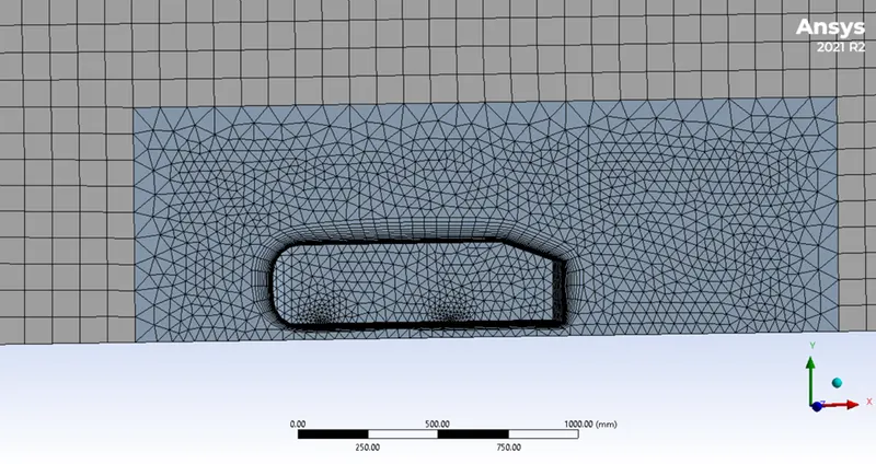
The first layer height came to be 0.44mm. We have selected the maximum number of layers = 20 and growth rate = 1.2. After adding the inflation layers the number of elements is 165092.

Below image shows the inflation layer in the model after meshing-

Pre-Processing and Solver Setting:

To compute the projection area for the car wall, go to projected areas under reports and compute it by selecting the direction (here, x) and name of the projected area (here, car wall).

Here, the projected area of car wall is 0.065741 and its length is 1.044m. These parameters we will have to input in reference values.

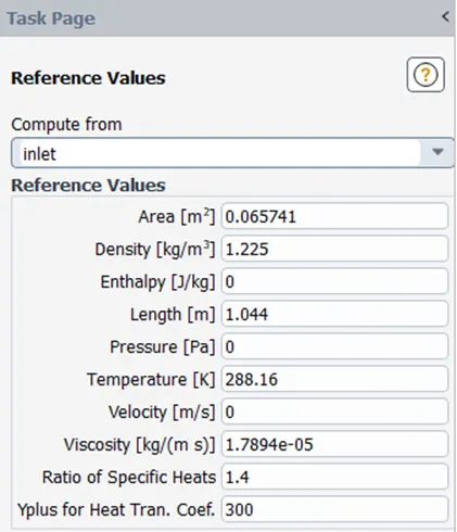
For Inlet, select type as velocity-inlet, click edit and enter the velocity as 25 m/s under the Momentum tab. And select the pressure-outlet for the outlet, since it is open to the atmosphere.

We have selected viscous model as K-epsilon for the solution. Now, select hybrid initialization and initialize and then run it for 500 iteration.

Now, for mesh independent study we have to run the simulation by changing the mesh size of the model and compare the results if it is changing significantly or not. If the results are very close to each other then we don’t need the smaller mesh size for the solution.

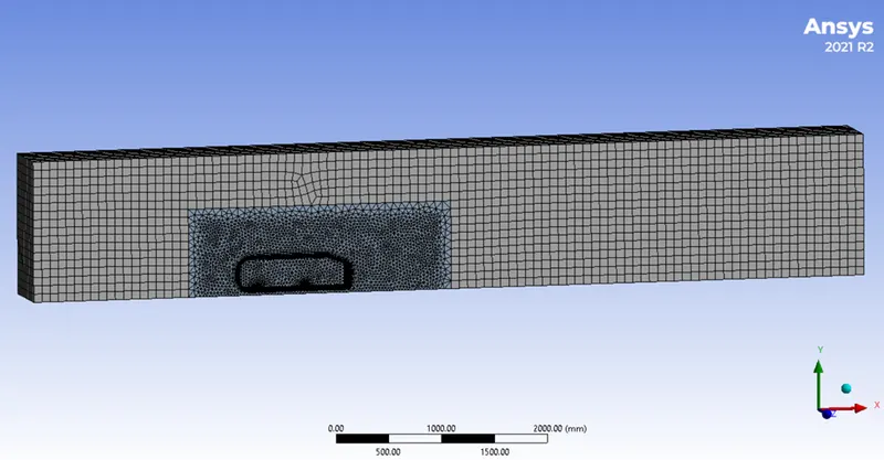
Case2-

Borderline mesh size= 80, inner enclosure mesh size= 30, number of elements= 312525.

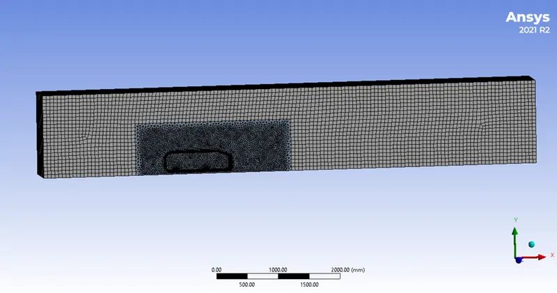
Case3-

Borderline mesh size= 60, inner enclosure mesh size= 25, number of elements= 520273.

The pre-processing and solver settings will not change in either of the cases.

Results-

The velocity contour plots for cases 1, 2 and 3 are shown below-

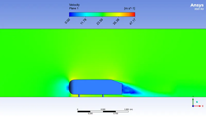
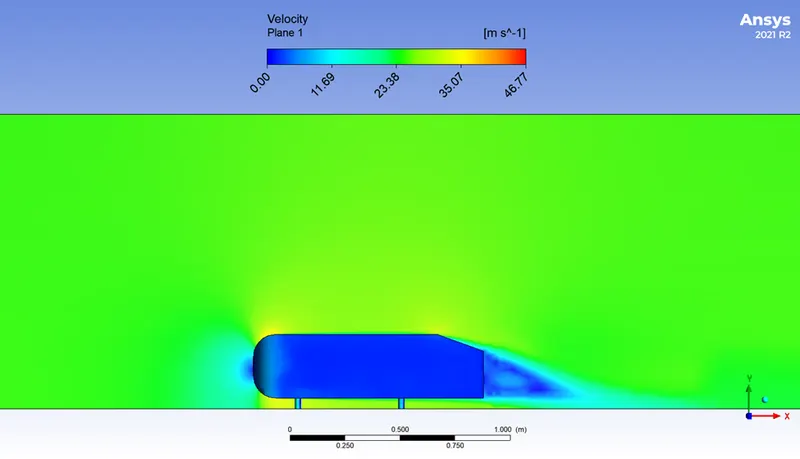
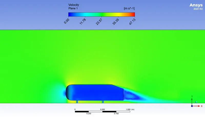
From the above images, you can see the wake region formation at the back of the Ahmed body.

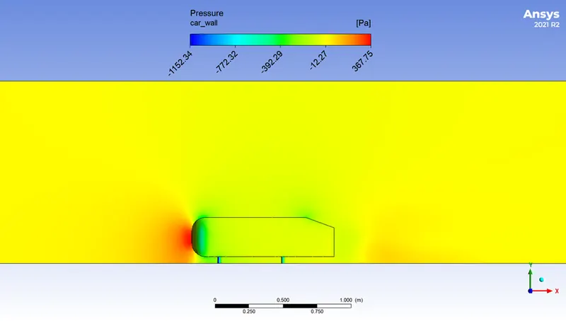
The pressure contour plots for cases 1, 2 and 3 are shown below-

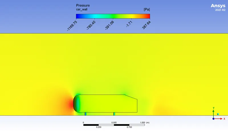
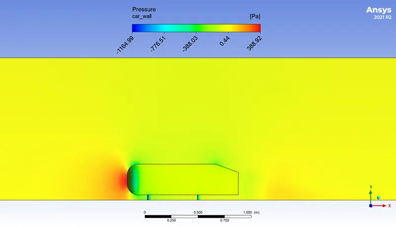
The drag coefficient plots for cases 1, 2 and 3 are shown below-

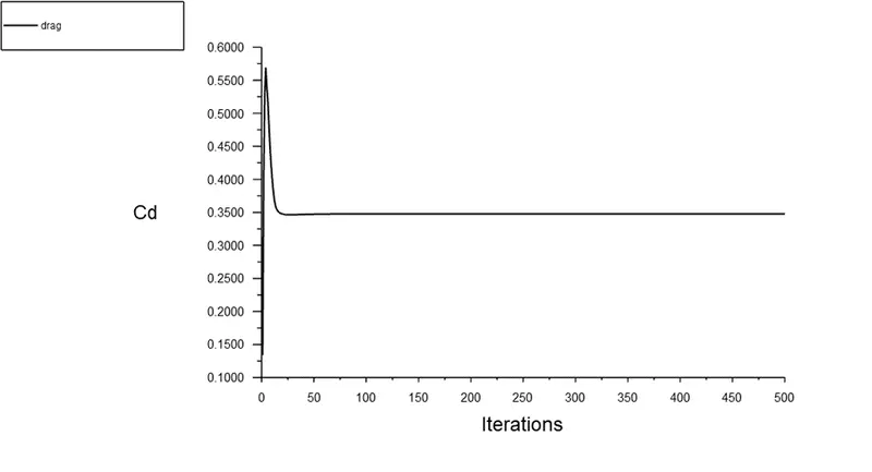
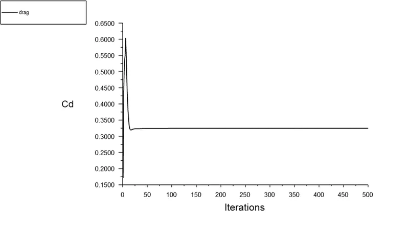
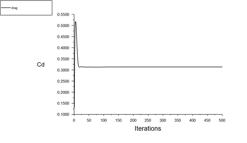
From the above images, you can see that all the graphs converged before 50 iterations. The values of the coefficients has been jotted down in a table in the conclusion.

The velocity vector and streamline plots for case 1 are shown below-

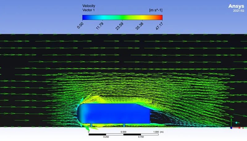
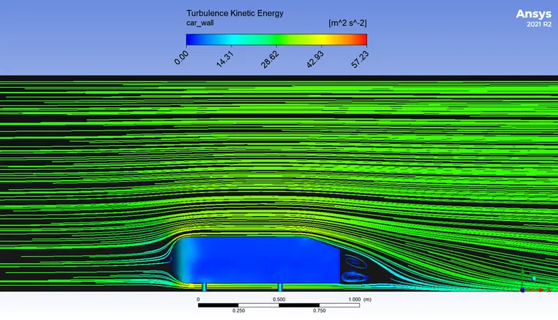
The above images clearly shows the formation of wake region at the back of the Ahmed body.

Conclusion-

Case no.	Base mesh size	Enclosure mesh size	No. of mesh elements	Drag coefficient	Lift coefficient
1	100	40	165092	0.3477016	0.289304
2	80	30	312525	0.3245541	0.2760471
3	60	25	520273	0.3132437	0.277101

As you can see from the above results of the mesh independent study, the difference in the drag and lift coefficients in case 2 and case 3 are very minute which means we don’t need to decrease the mesh element size further than the case 2.