Week 4.1 - Genetic Algorithm
Program using genetic algorithm to optimize stalagmite function and find global maxima.
Concept of Genetic Algorithm –
A Genetic Algorithm is a search heuristic that is inspired by Charles Darwin’s Theory of natural evolution. This algorithm reflects the process of natural selection where the fittest individual is selected for reproduction in order to produce offspring of the next generation.
It is a method for solving both constrained and unconstrained optimization problems that is based on natural selection. The algorithm begins by creating a random initial population of individual selections and it keeps on modifying this population repeatedly creating a sequence of new population. The algorithm uses the individuals in the current generation to create the next population. The genetic algorithm selects individuals at random from the current population to be parents and uses them to produce the children for the next generation. Over successive generations, the population evolves toward an optimal solution.
The genetic algorithm uses three main types of rules at each step to create the next generation from the current population:
- Selection rules select the individuals called parents, that contribute to the population at the next generation.
- Crossover rules combine two parents to form children for the next generation.
- Mutation rules apply random changes to individual parents to form children.
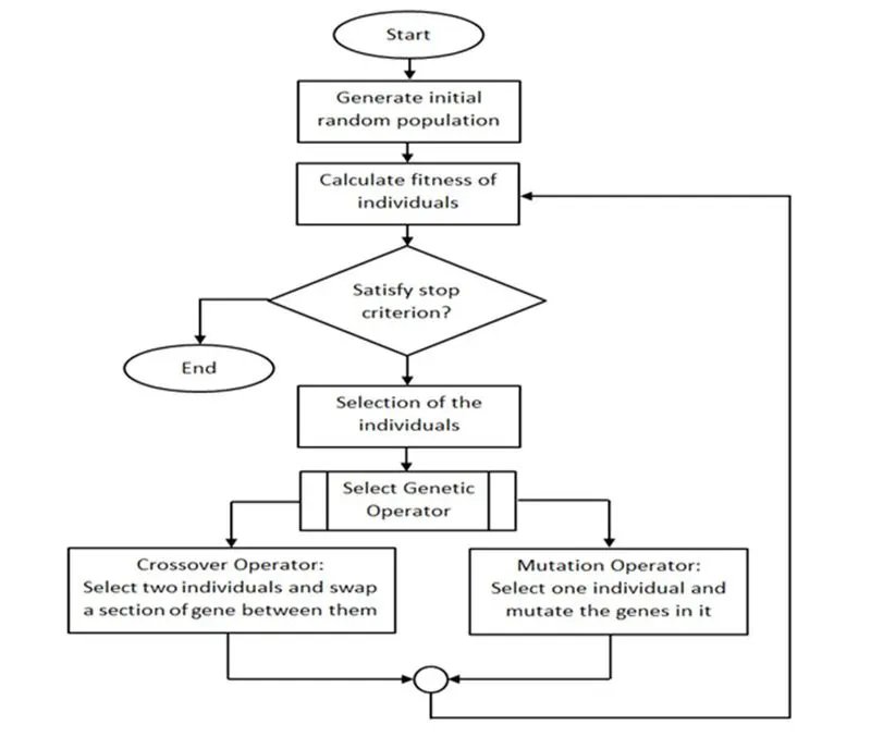
The basic steps in creating a genetic algorithm is as follows,
- The algorithm creates a random initial population at beginning.
- Then to create new population, the algorithm scores each member of the current population by computing its fitness value and converts them into a more usable range of values.
- Then based on these new values the algorithm selects members, called as parents.
- Then the algorithm produces children from the parents. Children are produced either by making random changes to a single parent which is mutation or by combining the vector entries of a pair of parents which is crossover.
- In this way the algorithm replaces the current population with the children to form the next generation.
- The algorithm stops when it reaches any one of the specified factors factors such as time limit, fitness limit, generations, function tolerance, constraint tolerance, etc.
The flowchart for Genetic Algorithm is given below,
Stalagmite function-
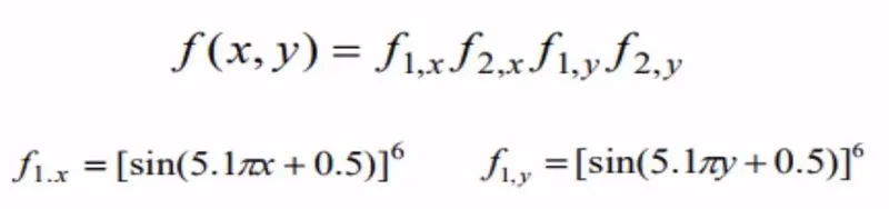
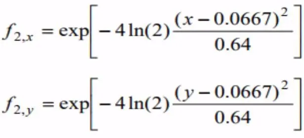
Stalagmite function is a mathematical model which helps to generate local minima and maxima. It is a three dimensional function and the way the function is designed is that it has a lot of local maxima or minima and one global maxima or minima. The name stalagmite is actually a type of rock formation that arises from the floor of a cave due to the accumulation of material deposited on the floor from ceiling drippings.
The stalagmite function is given as,
Syntax for defining ‘ga’ (Genetic Algorithm) in matlab –
The ‘ga’ syntax in matlab is used to find the minimum of function using genetic algorithm. There are several ways to define the ‘ga’ function depending on the problem being solved. The syntax used for this study is shown below.
- x = ga(fun,nvars)
where,
x = optimal solution/variables;
fun = Objective function;
nvars = Number of variables;
Sometimes ‘[x,fval]’ is used instead of ‘x’ where ‘fval’ gives objective function value in the solution.
- x = ga(fun,nvars,A,B,Aeq,Beq,lb,ub)
where,
A, B = Linear inequality constraints
Aeq, Beq = Linear equality constraints
If there are no linear equalities and inequalities, then A, B, Aeq, Beq are set to ‘[ ]’.
- x = ga(fun,nvars,A,B,Aeq,Beq,lb,ub,nonlcon,IntCon,options)
where,
nonlcon = Nonlinear constraints
IntCon = Integer Values
options = Optimization options
If there are no nonlinear constraints and integer values, the nonlcon and IntCon are set to ‘[ ]’.
Matlab code of stalagmite function-
function [sg] = stalagmite(input_vector)

x=input_vector(1);
y=input_vector(2);


t1 = pi*5.1*x;              % Equations are divided into different terms
t2 = pi*5.1*y;
t3 = ((x-0.0667)^2/0.64);
t4 = ((y-0.0667)^2/0.64);
t5 = (-4)*log(2);

xf1 = (sin(t1 + 0.5)).^6;       % Stalagmite functions

yf1 = (sin(t2 + 0.5)).^6;

xf2 = exp(t5*t3);

yf2 = exp(t5*t4);

sg = -(xf1*yf1*xf2*yf2);

end
Since we have to find the maxima of the function, we have put a negative sign in the function which will invert the stalagmite plot and show us the maxima.
MATLAB code to optimize the stalagmite function and find the Global Maxima of the function-
clear all
close all
clc

%% Defining our search engine
x = linspace(0,0.6,150);          % x - random input array
y = linspace(0,0.6,150);          % y - random input array
num_cases = 50;                   % number of iterations

%% Creating a 2D mesh array
[xx yy] = meshgrid(x,y);

%% Evaluating the stalagmite function
for i = 1:length(xx)
    for j = 1:length(yy)
        input_vector(1) =  xx(i,j);
        input_vector(2) =  yy(i,j);
        sg(i,j) = stalagmite(input_vector);      % calling the stalagmite function
    end
end

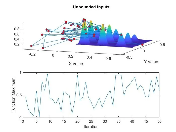
%% Study-1 - Statistical Behaviour (Unbounded condition)

tic                                              %tic and toc command is used for calculating the study time
for i = 1:num_cases
        [input, sg_opt(i)] = ga(@stalagmite,2);
        xopt(i) = input(1);
        yopt(i) = input(2);
end

study_1_time = toc

% Plotting the Graph
figure(1)
subplot(2, 1, 1)            % subplot - to have multiple plots in same figure window
hold on
surfc(x, y, -sg)
shading interp
plot3(xopt, yopt, -sg_opt, 'marker', 'o', 'markersize', 5, 'markerfacecolor', 'r')
title('Unbounded inputs')
xlabel('X-value')
ylabel('Y-value')
subplot(2, 1, 2)
plot(-sg_opt)
xlabel('Iteration')
ylabel('Function Maximum')

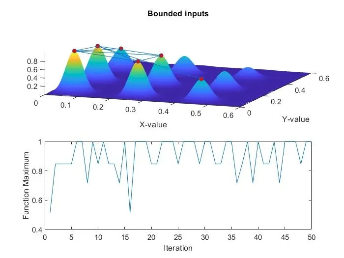
%% Study-2 - Statistical behaviour (with upper & lower bounds)

tic
for i = 1:num_cases
    [input, sg_opt(i)] = ga(@stalagmite, 2, [],[],[],[], [0;0], [1;1]);
        xopt(i) = input(1);
        yopt(i) = input(2);
end
study_2_time = toc

% Plotting the Graph
figure(2)
subplot(2, 1, 1)
hold on
surfc(x, y, -sg)
shading interp
plot3(xopt, yopt, -sg_opt, 'marker', 'o', 'markersize', 5, 'markerfacecolor', 'r')
title('Bounded inputs')
xlabel('X-value')
ylabel('Y-value')
subplot(2, 1, 2)
plot(-sg_opt)
xlabel('Iteration')
ylabel('Function Maximum')

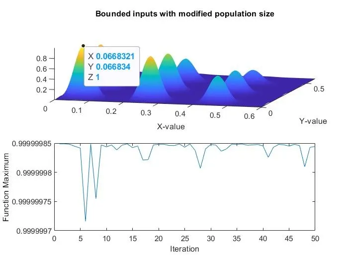
%% Study-3 - Increasing GA Iterations

options = optimoptions('ga');                              %Calculating the optimum solution for 'ga' and save in options(variable)
options = optimoptions(options, 'PopulationSize', 300);      % Increasing the size of the population to 300 to get accurate optimum result

tic
for i = 1:num_cases
    [input, sg_opt(i)] = ga(@stalagmite, 2, [],[],[],[], [0;0], [1;1], [], [], options);
        xopt(i) = input(1);
        yopt(i) = input(2);
end
study_3_time = toc

% Plotting the Graph
figure(3)
subplot(2, 1, 1)
hold on
surfc(x, y, -sg)
shading interp
plot3(xopt, yopt, -sg_opt, 'marker', 'o', 'markersize', 5, 'markerfacecolor', 'r')
title('Bounded inputs with modified population size')
xlabel('X-value')
ylabel('Y-value')
subplot(2, 1, 2)
plot(-sg_opt)
xlabel('Iteration')
ylabel('Function Maximum')
Most of the explanation is shown in the code itself. Somw explanation of the code are as follows-
- In this program we have did 3 studies for the genetic algorithm. In first study, the maximum value of function is found out with no restrictions, no bounds and no limits. The results of the first study will be different for each time we run the program.
- So, to get same value each time, we need to restrict the program within bounds ,i.e., upper bound and lower bound. The ‘ga’ syntax of this study will change as compared with the first study. This time the algorithm is provided lower limits and upper limits as [0;0] and [1;1] respectively.
- Now, after plotting the results for 2nd study, it is observed that the results are changing every time the program runs. A solution to this problem is to increase the number of cases or iterations.
- So, for the 3rd study, the number of iterations are increased to 300. The syntax of this study, “options = optimoptions(‘SolverName’,’Name’,‘Value’)” is used which returns with named parameter ‘Populations’ with the altered values ‘300’.
Results-